Chapter 21 ANOVA for randomised block designs

Block what you can; randomize what you cannot.

George Box

21.1 Randomized Complete Block Designs

We have only considered one type of experimental ANOVA design up until now: the Completely Randomised Design (CRD). The defining feature of a CRD is that treatments are assigned completely at random to experimental units. This is the simplest type of experimental design. Randomisation is a good thing because it prevents systematic biases creeping in. A CRD approach is often ‘good enough’ in many situations. However, it isn’t necessarily the most powerful design—if at all possible, we should use blocking to account for nuisance factors. A nuisance factor is one that has an effect on the response—it creates variation—but is of no interest to the experimenter. To end up with the most powerful experiment possible, the variability induced by nuisance factors should be accounted for at the design stage of an experiment. Let’s consider a hypothetical experiment to remind ourselves how blocking works…

Imagine we’re evaluating the effect of three different fertilizer application rates on wheat yields (t/ha). We suspect that the soil type and management histories of our experimental fields are quite different, leading to significant ‘field effects’ on yield. We don’t care about these field effects—they are a nuisance—but we’d like to account for them. There are two factors in play in this setting: the first is the set of treatments that are the subject of the experiment (fertilizer application rate); the second is the source of nuisance variation (field). Fertilizer application rate is the ‘treatment factor’ and field is the ‘blocking factor.’

Here is one way to block the experiment. The essence of the design is that a set of fields are chosen, which may differ in various unknown conditions (soil water, aspect, disturbance, etc.) and within each field, three plots are set up. Each plot receives one of the three fertilizer rate treatments at random. If we chose to work with eight fields the resulting data might look like this:

	Fertilizer	Control	Absent	High
Block	Field 1	9.3	8.7	10.0
	Field 2	8.7	7.1	9.1
	Field 3	9.3	8.2	10.4
	Field 4	9.5	8.9	10.0
	Field 5	9.9	9.1	10.8
	Field 6	8.9	8.0	9.0
	Field 7	8.3	6.2	8.9
	Field 8	9.1	7.0	8.1

Each treatment level is represented in each field (block), but only once. The experiment is ‘blocked by field.’ Now consider these two questions:

• Why is this design useful? Blocking allows us to partition out the environmental variation due to different field conditions. For example, the three treatments in field 5 produced a high yield relative to the yields within each treatment, while the yields in field 7 are consistently below average within each treatment. This among field variation is real, and if we hadn’t blocked the experiment and used a CRD it would manifest itself in the ‘noise’ component of our analysis. But since we blocked the experiment, and every treatment is present in every block, we can ‘remove’ the block variation from the noise. Less noise means more statistical power.

• Why is each treatment level is represented only once within blocks? This gives us the best chance of generalising our results. If we are interested in the overall effect of fertilizer, we should prefer to put our effort into including a range of possible environmental conditions. If we only did the experiment in one field the results might turn out to be rather unusual. We are not interested in the environmental variation as such, we just want to know for a range of conditions, whatever they might be, whether there are consistent differences between fertilizer application rates.

There are many different ways to introduce blocking into an experiment. The most commonly used design—and the one that is easiest to analyse—is called a Randomized Complete Block Design. The defining feature of this design is that each block sees each treatment exactly once. The fertiliser study is an example of a Randomized Complete Block Design (RCBD). The obvious question is: How do we analyse an RCBD? We’ll explore that after a small detour….

21.2 Designs without replication

So far we’ve only used the one-way ANOVA. As we’ll find out in the Introduction to two-way ANOVA chapter we can have more than one treatment in an ANOVA. Usually when we’re interested in the effect of two variables on our response variable we’ll have the following design: two factors, each having two or more levels, with replicate measurements within each combination of levels:

	Factor A	Level 1	Level 2	Level 3
Factor B	Level 1	1,2,3	1,5,9	2,6,8
	Level 2	3,4,2	…	…
	Level 3	4,7,9	…	…
	Level 4	4,6,5	…	…

As we have just seen however, it is possible to have a two-way design with only a single measurement within each combination of levels:

	Factor A	Level 1	Level 2	Level 3
Factor B	Level 1	1	1	2
	Level 2	3	…	…
	Level 3	4	…	…
	Level 4	2	…	…

What’s this… no replication? Isn’t that a problem? In fact there is replication of a sort for each level of the factors. For example there are 3 values for each level of Factor B, it’s just that each value is at a different level of Factor A. This means we can still compare the means for the different levels of each treatment using an ANOVA (that is, we can analyse the main effects). What we can’t do is determine whether the effect of Factor B varies depending on the value of Factor A. This is called the interaction. We’ll come back to this idea in the Introduction to two-way ANOVA chapter so don’t worry if it seems confusing now.

So… it is possible to carry out a two-way ANOVA without replication, even though we can’t learn anything about that mysterious interaction with this sort of design. Is this useful? Yes—it is useful when one one of the factors is a blocking factor. If our experimental design has a single blocking factor and one treatment factor, and we adopt an RCBD, this leads to an unreplicated two-way arrangement. The fact that we can’t estimate an interaction is not a problem. In fact, “it’s a feature, not a bug.” We only need to know about the average effect of each treatment (across blocks) to be able to generalise our results, and we can definitely estimate that.

So there is nothing “dodgy” about a two-way design without replication. Indeed, it is the best design to use in some situations, such as an RCBD experiment. Let’s see how to the analyse a Randomized Complete Block Design experiment.

21.3 Analysing an RCBD experiment

Let’s consider a new example to really drive home how an RCBD works. We want to assess whether there is a difference in the impact that the predatory larvae of three damselfly species (Enallagma, Lestes and Pyrrhosoma) have on the abundance of midge larvae in a pond. We plan to conduct an experiment in which small (1 m²) nylon mesh cages are set up in the pond. All damselfly larvae will be removed from the cages and each cage will then be stocked with 20 individuals of one of the species. After 3 weeks we will sample the cages and count the density of midge larvae in each. We have 12 cages altogether, so four replicates of each of the three species can be established.

On the face of it this looks like a straightforward one-way design, with each species as a treatment. The only problem to resolve is how to distribute the enclosures in the pond. Obviously the pond is unlikely to be uniform in depth, substrate, temperature, shade, etc… Some of the variation will be obvious, some will not. We have two options: 1) use a CRD and distribute the cages at random, or 2) adopt an RCBD by grouping the cages into clusters of three, placing each cluster at a randomly chosen location, and assigning the three treatments to cages at random within each cluster. These are illustrated below (left = CRD, right = RCBD):

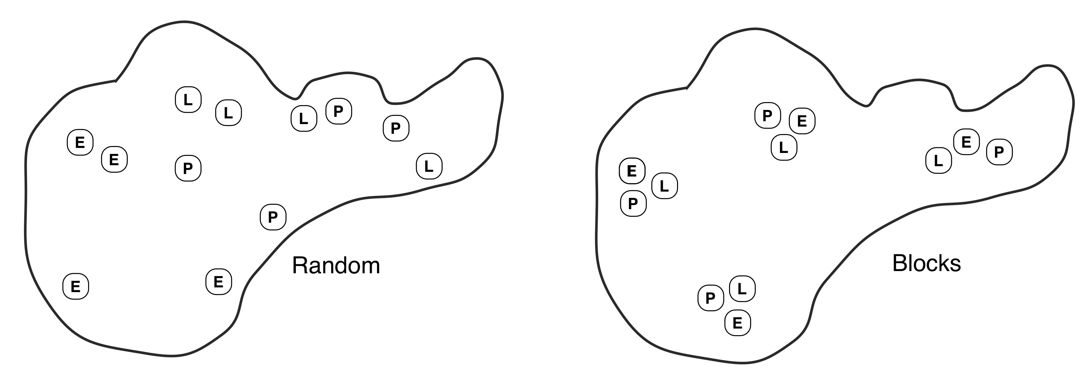
What are the consequences of the two alternatives? If the cages are distributed at random (CRD) then they will cover a wide range of variation in these various factors. These sources of variation will almost certainly cause the density of midge larvae to vary around the pond in an unpredictable way, increasing the noise in the data. If we group sets of treatments into clusters we are creating ‘spatial blocks.’ There may be considerable differences between blocks, but these won’t obscure differences between the treatments because all three treatments are present in every block.

21.4 Carrying out the analysis with R

Walk through example

You should work through the example from here.

The data from the damselfly experiment are in a file called DAMSELS.CSV.

damsels <- read_csv("./DAMSELS.CSV")

glimpse(damsels)

## Rows: 12
## Columns: 3
## $ Midge   <dbl> 304, 464, 320, 578, 509, 458, 680, 740, 630, 356, 390, 350
## $ Species <chr> "Enallagma", "Lestes", "Pyrrhosoma", "Enallagma", "Lestes", "…
## $ Block   <chr> "A", "A", "A", "B", "B", "B", "C", "C", "C", "D", "D", "D"

The density of midge larvae in each enclosure, after running the experiment for 3 weeks, are in the Midge variable (number m\(^{-2}\)); codes for species in the Species variable (levels: Enallagma, Lestes and Pyrrhosoma), and the block identities (A, B, C, D) in the third column.

The process of analysing an RCBD is essentially the same as any other type of ANOVA. First we fit the model using the lm function and then we use anova to calculate F-statistics, degrees of freedom, and p-values:

damsels.model <- lm(Midge ~ Species + Block, data = damsels)
anova(damsels.model)

We suppressed the output for now. Notice that we have put two factors on the right hand side of the ~ symbol. This tells R that we want to fit a model that accounts for the main effects of Species and Block. We put a + between terms to delineate them.

Careful with your + and *

Notice that we set up the blocking factor in the model using the ‘plus’ symbol: Species + Block. R also allows us to use the ‘times’ symbol inside a model formula, e.g. Species Block. You will see this used later when we get to two-way designs. However, you should use + to include a blocking factor like Block in a model as a so-called ‘main effect’ term. We’ll talk about what that means later. For now, just note that blocking factors are included via +.

And by the way… the + has nothing to do with addition when working with model specifications in R.

Here are the results of the global significance tests using the correct ANOVA model for our randomised block experiment:

anova(damsels.model)

## Analysis of Variance Table
## 
## Response: Midge
##           Df Sum Sq Mean Sq F value    Pr(>F)    
## Species    2  14904    7452  3.0053 0.1246687    
## Block      3 208425   69475 28.0182 0.0006306 ***
## Residuals  6  14878    2480                      
## ---
## Signif. codes:  0 '***' 0.001 '**' 0.01 '*' 0.05 '.' 0.1 ' ' 1

What does all this mean? We interpret each line of the ANOVA table in exactly the same way as we do for a one-way ANOVA. The first part tells us what kind of output we are looking at:

## Analysis of Variance Table 
##  
## Response: Midge

This reminds us that we are looking at an ANOVA table where our response variable was called Midge. The table contains the key information:

##           Df Sum Sq Mean Sq F value    Pr(>F)     
## Species    2  14904    7452  3.0053 0.1246687     
## Block      3 208425   69475 28.0182 0.0006306 *** 
## Residuals  6  14878    2480

This ANOVA table is similar to the ones we have already seen, except that now we have to consider two lines—one for each term in the model. The first is for the main effect of Species and the second for the main effect of Block.

The F-ratio is the test statistic for each term. These provides a measure of how large and consistent the effects associated with each term are. Each F-ratio has a pair of degrees of freedom associated with it: one belonging to the term itself, the other due to the error (residual). Together, the F-ratio and its degrees of freedom determines the p-value.

The p-value gives the probability that the differences between the set of means for each term in the model, or a more extreme difference, could have arisen through sampling variation under the null hypothesis of no difference. We take p < 0.05 as evidence that at least one of the treatments is having an effect. Here, there is a significant effect of block (p < 0.001), which says that the density of midge larvae varies across the lake. It looks like blocking was a good idea—there is a lot of spatial (nuisance) variation in midge larvae density. Of course what we actually care about is the damselfly species effect. This main effect term is not significant (p > 0.05), so we conclude that there is no difference in the impact of the predatory larvae of three damselfly species.

It is worth looking at what happens if we analyse the damselfly data as though they are from a one-way design. We do this by including only the experimental treatment term (Species) in the model:

damsels.oneway <- lm(Midge ~ Species, data = damsels)
anova(damsels.oneway)

## Analysis of Variance Table
## 
## Response: Midge
##           Df Sum Sq Mean Sq F value Pr(>F)
## Species    2  14904  7452.1  0.3003 0.7477
## Residuals  9 223303 24811.4

Look at the degrees of freedom and the sums of squares of the residual (error). How do these compare to the previous model that accounted for the block effect? The degrees of freedom is higher. In principle this is a good thing because it means we have more power to detect a significant difference among the treatment means. However, the error sum of squares is also much higher when we ignore the block effect. We have accounted for much less noise by ignoring the block effect. As a result, the error mean square is much lower, and so the F-statistic associated with the treatment effect is also much lower. The take home message is that designing a blocked experiment, and properly accounting for the blocked structure, will (usually) result in a more powerful analysis.

21.4.1 Multiple comparisons anyone?

In a randomised block analysis we are not usually interested in investigating significant block effects—the primary role of the blocking is to remove unwanted variation that might obscure the differences between treatments. R automatically gives us a test of the block effect, and if it is significant it tells us that using the block layout has removed a considerable amount of variation (though even if the result isn’t quite what would conventionally be regarded as significant, i.e. if is not as low as 0.05, then the blocking may still have been helpful). For this, and other, technical reasons we never carry out multiple comparisons between the block means. If the treatment effect is significant, multiple comparisons can be done between the treatment means using the Tukey test.

21.5 Are there disadvantages to randomised block designs?

The short answer is no, not really. There are instances when a randomised block design might appear to be disadvantageous at first glance, but these don’t really stand up to criticism:

1. What if we were interested in knowing whether there is an interaction between the levels of the block and the treatments? For example, in the damselfly experiment we might be interested to know whether, if the damselfly species have differing effects on the midge densities, these effects are consistent in all habitat areas (e.g. some species may forage more effectively in muddy areas, others where there are more leaves). If this is the question we are trying to answer, then we should really have designed a different experiment. For example, a two-way design (which might also include blocking) in which we consider treatment combinations of different midge species and habitat characteristics might be appropriate. Fundamentally, the goal of blocking is to account for uncontrolled variation. Designing a blocked experiment and then lamenting the fact that we can’t fully evaluate differences among blocks is a good example of trying to “have our cake and eat it too.”

2. If the blocking term is having no effect in accounting for some of the variation, then the analysis may be slightly less powerful than just using a one-way ANOVA. This is because there are fewer error degrees of freedom associated with the blocked analysis (we lose a few to the block effects). This argument only works if the block effect accounts for very little variation. We can never know before we start an experiment whether or not blocking is needed, but we do know that biological systems are inherently noisy, with many sources of uncontrolled variation coming into play. In the majority of experimental settings (in biology at least) we can be fairly sure that blocking will ‘work.’ If we choose not to block an experiment there is no way to account for uncontrolled variation and we will almost certainly end up losing statistical power as a result.

The advice contained in the quote at the beginning of this chapter is probably the best experimental design advice ever dished out: “Block what you can; randomize what you cannot.”

21.6 Multiple blocking factors

It is common to find ourselves in a situation whereby we need to account for more than one blocking factor. The simplest option is to combine the nuisance factors into a single factor. However, this isn’t always possible, or even desirable. Consider an instance where there is a single factor of primary interest (the treatment factor) and two nuisance factors. For example, imagine that we want to test three drugs A, B, C for their effect in alleviating the symptoms of a disease. Three patients are available for a trial, and each will be available for three weeks. Testing a single drug requires a week, meaning an experimental unit is a ‘patient-week.’ The obvious question is, how should we randomise treatments across ‘patient-weeks?’

We have to design an experiment like this with great care, or there is a risk that we will not be able to statistically separate the effects of the treatment (drug) and block effects (week & patient). The most appropriate design for this kind of experiment has the following structure:

	Week	Patient	Drug
	1	1	A
	1	2	B
	1	3	C
	2	1	C
	2	2	A
	2	3	B
	3	1	B
	3	2	C
	3	3	A

This kind of experimental design is called a Latin square design. It gets its name form the fact that if we organise the treatments into the rows and columns of a grid according to week and patient number, we arrive at something like this¹⁷:

A   B   C
C   A   B
B   C   A

Notice that each letter appears once in each column and row. Mathematicians call this a Latin square arrangement. Latin square designs (and their more exotic friends, e.g. ‘Hyper-Graeco-Latin square designs!’) have a very useful property: they allow us to unambiguously separate treatment and block effects. The reasoning behind this conclusion is quite technical, so we won’t try to explain it. We just want to demonstrate that it is perfectly possible to block an experiment by more than one factor, but this needs to be done with care (this is a ‘seek advice’ situation).