Chapter 17 Introduction to one-way ANOVA

17.1 Introduction

The two-sample t-tests evaluate whether or not the mean of a numeric variable changes among two groups or experimental conditions, which can be encoded by a categorical variable. We can conceptualise this test as one that evaluates whether or not the numeric variable is related to the categorical variable, reflected as a difference between means of different groups. The obvious question is, what happens if we need to evaluate differences among means of more than two groups? The ‘obvious’ thing to do might seem to be to test each pair of means using a t-test. However this procedure is statistically flawed.

In this chapter, we will introduce a new method to assess the statistical significance of differences among several means at the same time. This is called Analysis of Variance (abbreviated to ANOVA). ANOVA is one of those statistical terms that unfortunately has two slightly different meanings:

In its most general sense ANOVA refers to a methodology for evaluating statistical significance. It appears when working with a statistical model known as the ‘general linear model.’ Simple linear regression is one special case of the general linear model. Whenever we see an F-ratio in a statistical test we’re carrying out an Analysis of Variance of some kind.
In its more narrow sense the term ANOVA is used to describe a particular type of statistical model. When used like this ANOVA refers to models that compare means among two or more groups. The various types of ANOVA models are also special cases of general linear models. The ANOVA-as-a-model is the focus of this chapter.

ANOVA models underpin the analysis of many different kinds of experimental data; they are one of the main ‘work horses’ of basic data analysis. As with many statistical models we can use ANOVA without really understanding the details of how it works. However, when it comes to interpreting the results of statistical tests associated with ANOVA, it is important to at least have a basic conceptual understanding of how it works. The goal of this chapter is to provide this basic understanding. We’ll do this by exploring the simplest type of ANOVA model: One-way Analysis of Variance.

One-way Analysis of Variance allows us to predict how the mean value of a numeric variable (the response variable) responds or depends on the values of a categorical variable (the predictor variable). This statement is just another way of way of saying that the ANOVA model compares means among groups defined by the categorical variable. It is no coincidence that this sounds a lot like our description of simple regression. ANOVA and regression are both special cases of the general linear model. This observation explains why…

regression and ANOVA can be described with a common language (e.g. response vs predictor variables), and
the workflows for developing ANOVA and regression analyses are actually very similar in terms of what we have to do in R.

17.2 Why do we need ANOVA models?

The corncrake, Crex crex, underwent severe declines in the UK thought to be due to changes in farming practices. Captive breeding and reintroduction programmes were introduced to try to help supplement the wild population. The scientists in charge of the breeding programme wanted to determine the success of 4 different supplements (the predictor variable) for increasing initial growth (the response variable) in the captively bred hatchlings. They conducted an experiment in which groups of 8 hatchlings were fed with different supplements. A fifth group of 8 hatchlings served as the control group—they were given the base diet with no supplements. At the end of the experiment they measured how much weight each hatchling had gained over the week.

We can plot the weight gain of 8 hatchlings on each of the supplements (this is the raw data), along with the means of each supplement group, the standard error of the mean, and the sample mean of all the data:

## `summarise()` ungrouping output (override with `.groups` argument)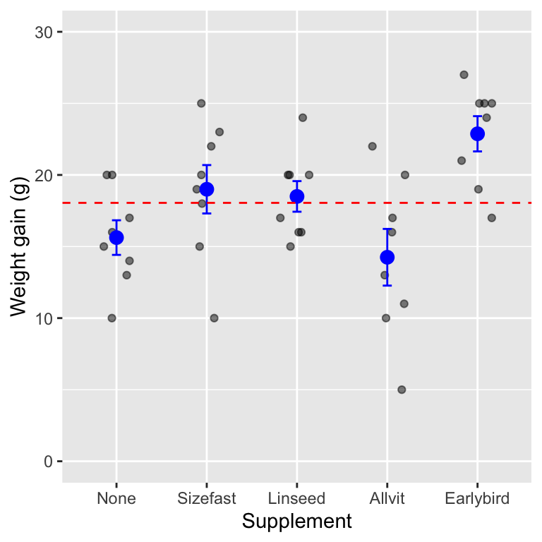

The grey points are the raw data, the means and standard error of each group are in blue, and the overall sample mean is shown by the dashed red line. We can see that there seem to be differences among the means: hatchlings in each of the different groups often deviate quite a lot from the overall average for all of the hatchlings in the study (the dashed line). This would seem likely to be an effect of the supplements they are on. At the same time, there is still a lot of variation within each of the groups: not all of the hatchlings on the same supplements has the same weight gain.

Perhaps all of this could be explained away as sampling variation—i.e. the supplements make no difference at all to weight gain. Obviously we need to apply a statistical test to decide whether these differences are ‘real.’

It might be tempting to use t-tests to compare each mean value with every other. However, this would involve 10 t-tests. Remember, if there is no effect of supplement, each time we do a t-test there is a chance that we will get a false significant result. If we use the conventional p = 0.05 significance level, there is a 1 in 20 chance of getting such ‘false positives.’ Doing a large number of such tests increases the overall risk of finding a false positive. In fact doing ten t-tests on all possible comparisons of the 5 different supplements gives about 40% chance of at least one test giving a false significant difference, even though each individual test is conducted with p = 0.05.

That doesn’t sound like a very good way to do science. We need a reliable way to determine whether there is a significance of differences between several means without increasing the chance of getting a spurious result. That’s the job of Analysis of Variance (ANOVA). Just as a two sample t-test compares means between two groups, ANOVA compares means among two or more groups. The fundamental job of an ANOVA model is to compares means. So why is it called Analysis of Variance? Let’s find out…

17.3 How does ANOVA work?

The key to understanding ANOVA is to realise that it works by examining the magnitudes of different sources of variation in the data. We start with the total variation in the response variable—the variation among all the units in the study—and then partition this into two sources:

Variation due to the effect of experimental treatments or control groups. This is called the ‘between-group’ variation. This describes the variability that can be attributed to the different groups in the data (e.g. the supplement groups). This is the same as the ‘explained variation’ described in the Relationships and regression chapter. It quantifies the variation that is ‘explained’ by the different means.
Variation due to other sources. This second source of variation is usually referred to as the ‘within-group’ variation because it applies to experimental units within each group. This quantifies the variation due to everything else that isn’t accounted for by the treatments. Within-group variation is also called the ‘error variation.’ We’ll mostly use this latter term because it is a bit more general.

ANOVA does compare means, but it does this by looking at changes in variation. That might seem odd, but it works! If the amount of variation among treatments is sufficiently large compared to the within-group variation, this suggests that the treatments are probably having an effect. This means that in order to understand ANOVA we have to keep three sources of variation in mind: the total variation, the between-group variation, and the error variation.

We’ll get a sense of how this works by carrying on with the corn crake example. We’ll look at how to quantify the different sources of variation, and then move on to evaluate statistical significance using these quantities. The thing to keep in mind is that the logic of these calculations is no different from that used to carry out a regression analysis. The only real difference is that instead of fitting a line through the data, we fit means to different groups when working with an ANOVA model.

Total variation

The figure below shows the weight gain of each hatchling in the study and the grand mean (i.e. we have not plotted the group-specific means).

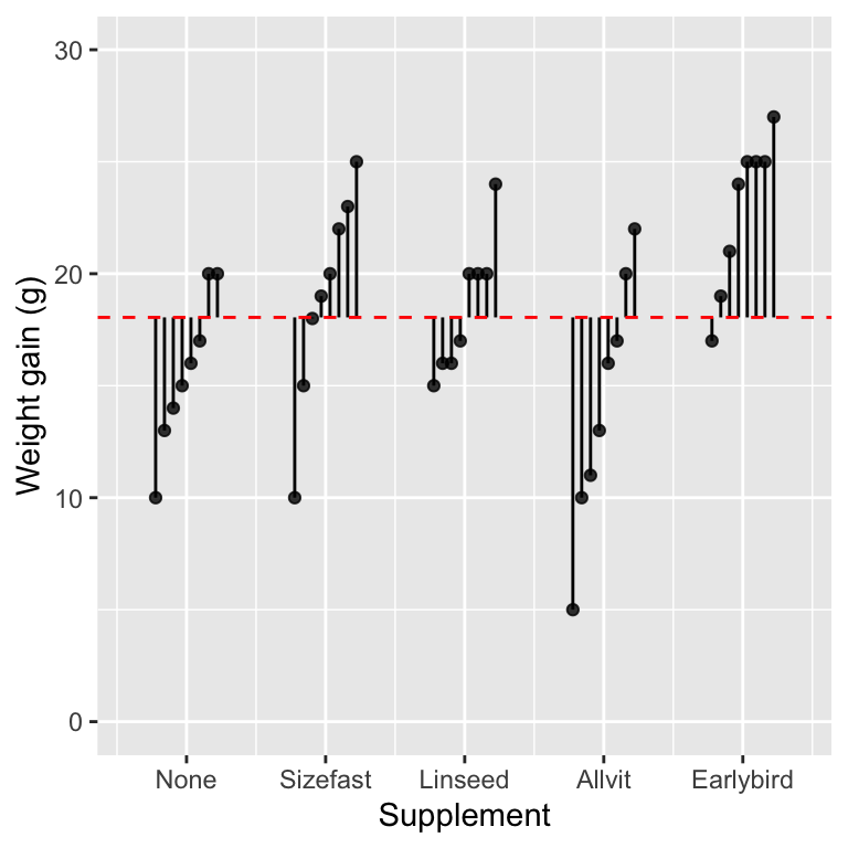
The vertical lines show the distance between each observation and the grand mean—we have ordered the data within each group so that the plot is a little tidier. A positive deviation occurs when a point is above the line, and a negative deviation corresponds to a case where the point is below the line. We’re not interested in the direction of these deviations. What we need to quantify is the variability of the deviations, which is a feature of their magnitude (the length of the lines).

What measure of variability should we use? We can’t add up the deviations because they add to zero. Instead, we apply the same idea introduced in the Relationships and regression chapter: the measure of variability we need is based on the ‘sum of squares’ (abbreviated SS) of the deviations. A sum of squares is calculated by taking each deviation in turn, squaring it, and adding up the squared values. Here are the numeric values of the deviations shown graphically above:

##  [1]  -5.05   1.95  -1.05  -2.05  -3.05  -4.05  -8.05   1.95  -3.05  -0.05
## [11]  -8.05   3.95   4.95   0.95   6.95   1.95   1.95   5.95  -1.05  -2.05
## [21]   1.95   1.95  -3.05  -2.05   3.95 -13.05  -8.05  -2.05  -7.05  -1.05
## [31]   1.95  -5.05  -1.05   6.95   5.95   6.95   6.95   0.95   8.95   2.95

The sum of squares of these numbers is 967.9. This is called the total sum of squares, because this measure of variability completely ignores the information about treatment groups. It is a measure of the total variability in the response variable, calculated relative to the grand mean.

Residual variation

The next component of variability we need relates to the within-group variation. Let’s replot the original figure showing the weight gain of each hatchling (points), the mean of each supplement group (horizontal blue lines), and the grand mean:

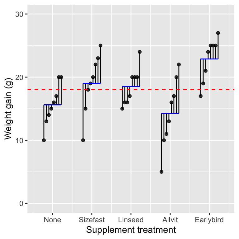
The vertical lines show something new this time. They display the distance between each observation and the group-specific means, which means they summarise the variation among hatchlings within treatment groups. Here are the numeric values of these deviations:

##  [1] -9.250 -5.625 -9.000 -4.250 -3.250 -2.625 -1.250 -1.625 -0.625 -4.000
## [11] -3.500  0.375 -2.500 -2.500  1.750  1.375 -1.500  2.750 -5.875 -1.000
## [21]  0.000 -3.875  4.375  4.375  1.000  1.500  1.500  1.500  5.750 -1.875
## [31]  3.000  7.750  4.000  5.500  1.125  6.000  2.125  2.125  2.125  4.125

These values are a type of residual: they quantify the variation that is ‘left over’ after accounting for differences due to treatment groups. Once again, we can summarise this variability as a single number by calculating the associated sum of squares, calculated by taking each deviation in turn, squaring it, and adding up the squared values. The sum of squares of these numbers is (610.25). This is called the residual sum of squares¹⁰. It is a measure of the variability that may be attributed to differences among individuals after controlling for the effect of different groups.

Between-group variation

The last component of variability we need relates to the between group variation. We’ll replot the figure one more time, but this time we’ll show just the group-specific means (blue points), the overall grand mean (dashed red line), and the deviations of each group mean from the grand mean:

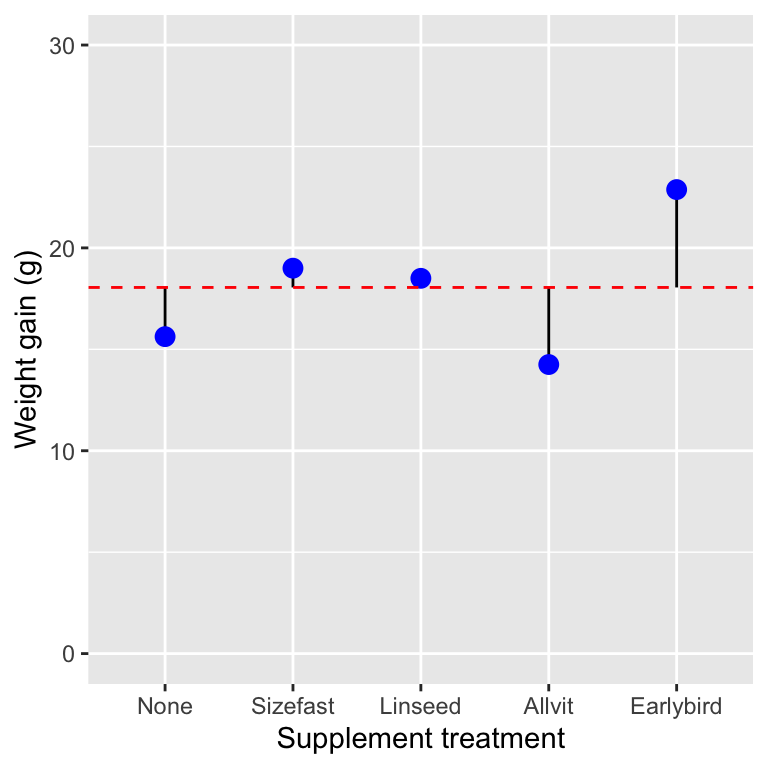
Now the vertical lines show the distance between each group-specific mean and the grand mean. We have five different treatment groups, so there are only five lines. These lines show the variation due to differences among treatment groups. Here are the numeric values of these deviations:

## [1] -2.425  0.950  0.450 -3.800  4.825

These values quantify the variation that can be attributed to differences among treatments. Once again, we can summarise this variability as a single number by calculating the associated sum of squares—this number is called the treatment sum of squares. This is the same as the ‘explained sum of squares’ discussed in the context of regression. It is a measure of the variability attributed to differences among treatments.

This is 44.71 in the corn crake example. Notice that this is much smaller than the total sum of squares and the residual sum of squares. This isn’t all that surprising as it is based on five numbers, whereas the other two measures of variability are based on all the observations.

17.3.1 Degrees of freedom

The problem with the raw sums of squares in ANOVA is that they are a function of sample size and the number of groups. In order to be useful, we need to convert them into measures of variability that don’t scale with sample size. We use degrees of freedom (written as df, or d.f.) to do this. We came across the concept of degrees of freedom when we studied regression: the degrees of freedom associated with a sum of squares is a measure of how much ‘information’ it is based on. Each of the three sums of squares we just calculated has a different degrees of freedom calculation associated with it:

Total d.f. = (Number of observations - 1)
Treatment d.f. = (Number of treatment groups - 1)
Error d.f. = (Number of observations - Number of treatment groups)

The way to think about these is as follows. We start out with a degrees of freedom that is equal to the total number of deviations associated with a sum of squares. We ‘lose’ one degree of freedom for every mean we have to calculate to work out the deviations. Here is how this works in the corn crake example:

Total d.f. = 40 - 1 = 39 — The total sum of squares was calculated using all 40 observations in the data, and the deviations were calculated relative to 1 mean (the grand mean).
Treatment d.f. = 5 - 1 = 4 — The treatment sum of squares was calculated using the 5 treatment group means, and the deviations were calculated relative to 1 mean (the grand mean).
Error d.f. = 40 - 5 = 35 — The error sum of squares was calculated using all 40 observations in the data, and the deviations were calculated relative to 5 means (the treatment group means).

Don’t worry too much if that seems confusing. We generally don’t have to carry out degrees of freedom calculations by hand because R will do them for us. We have explained them because knowing where they come from helps us understand the output of an ANOVA significance test.

17.3.2 Mean squares, variance ratios, and F-tests

Once we know how to calculate the degrees of freedom we can use them to standardise each of the sums of squares. The calculations are very simple. We take each sum of squares and divide it by its associated degrees of freedom. The resulting quantity is called a mean square (abbreviated as MS): \[ \text{Mean square} = \frac{\text{Sum of squares}}{\text{Degrees of freedom}} \] We stated what a mean square represents when discussing regression: it is an estimate of a variance. The mean squares from an ANOVA quantify the variability of the whole sample (total MS), the variability explained by treatment group (treatment MS), and the unexplained residual variation (residual MS).

ANOVA quantifies how strong the treatment effect is by comparing the treatment mean square to the residual mean square. When the treatment MS is large relative to the residual MS this suggests that the treatments are more likely to be having an effect. In reality, they are compared by calculating the ratio between them (designated by the letter F):

\[F = \mbox{Variance ratio} = \frac{\mbox{Variance due to treatments}}{\mbox{Error variance}}\]

This is the same as the F-ratio mentioned in the context of regression. When the variation among treatment means (treatment MS) is large compared to the variation due to other factors (residual MS) then the F-ratio will be large too. If the variation among treatment means is small relative to the residual variation then the F-ratio will be small. How do we decide when the F-ratio is large enough? That is, how do we judge a result to be statistically significant? We play out the usual ‘gambit’:

We assume that there is actually no difference between the population means of each treatment group. That is, we hypothesise that the data in each group are sampled from a single population with one mean.
Next, we use information in the sample to help us work out what would happen if we were to repeatedly take samples in this hypothetical situation. The ‘information’ in this case are the mean squares.
We then ask, ‘if there is no difference between the groups, what is the probability that we would observe a variance ratio that is the same as, or more extreme than, the one we actually observed in the sample?’
If the observed variance ratio is sufficiently improbable, then we conclude that we have found a ‘statistically significant’ result, i.e. one that is inconsistent with the hypothesis of no difference.

In order to work through these calculations we make one key assumption about the population from which the data in each treatment group has been sampled. We assume that the residuals are normally distributed. Once we make this assumption the distribution of the F-ratio under the null hypothesis (the ‘null distribution’) has a particular form: it follows an F distribution. This means we assess the statistical significance of differences between means by comparing the F-ratio calculated from a sample of data to the theoretical F distribution.

This procedure is a type of F-test—it is really no different from the significance testing methodology outlined for regression models. The important message is that ANOVA works by making just one comparison: the treatment variation and the error variation, rather than the ten t-tests that would have been required to compare all the pairs.

17.4 Different kinds of ANOVA model

There are many different flavours of ANOVA model. The one we’ve just been learning about is called a one-way ANOVA. It’s called one-way ANOVA because it involves only one factor: supplement type (this includes the control). If we had considered two factors—e.g. supplement type and amount of food—we would have to use something called a two-way ANOVA. A design with three factors is called a three-way ANOVA, and… you get the idea.

There are many other ANOVA models, each of which is used to analyse a specific type of experimental design. We are only going to consider three different types of ANOVA in this book: one-way ANOVA, two-way ANOVA, and ANOVA for one-way, blocked design experiments.

17.5 Some common questions about ANOVA

To finish off with, three common questions that often arise:

17.5.1 Can ANOVA only be applied to experimental data?

We have been discussing ANOVA in the context of a designed experiment (i.e. we talked about treatments and control groups). Although ANOVA was developed to analyse experimental data—and that is where it is most powerful—it can be used in an observational setting. As long as we’re careful about how we sample different kinds of groups (i.e. at random), we can use ANOVA to analyse differences between them. The main difference between ANOVA for experimental and observational studies arises in the interpretation of the results. If the data aren’t experimental, we can’t say anything concrete about the causal nature of the among-group differences we observe.

17.5.2 Do we need equal replication?

So far we have only considered the use of ANOVA with data in which each treatment has equal replication. One of the frequent problems with biological data is we often don’t have equal replication, even if we started with equal replication in our design. Plants and animals have a habit of dying before we have gathered all our data; a pot may get dropped, a culture contaminated, all sorts of things conspire to upset even the best designed experiments. Fortunately one-way ANOVA does not require equal replication, it will work even where sample sizes differ between treatments.

17.5.3 Can ANOVA be done with only two treatments?

Although the t-test provides a convenient way of testing means from two treatments, there is nothing to stop you doing an ANOVA on two treatments. A t-test (assuming equal variances) and ANOVA on the same data should give the same p-value (in fact the F-statistic from the ANOVA will be the square of the t-value from the t-test). One advantage to the t-test, however, is that you can do the version of the test that allows for unequal variances—something a standard ANOVA does not do. There is a version of Welch’s test for one-way ANOVA, but we won’t study it in this course (look at the oneway.test function if you are interested).

You will sometimes see something called error sum of squares, or possibly, the within-group sum of squares. These are just different names for the residual sum of squares.↩︎