Chapter 7 Sampling error

In the previous chapter we introduced the idea that point estimates of a population parameter are always imperfect, in that they won’t exactly match its true value. This uncertainty unavoidable. This means it is not enough to have estimated something–we have to also know about the uncertainty of the estimate. We use the machinery of statistics to quantify this uncertainty.

Once we have pinned down the uncertainty we can start to provide meaningful answers to our scientific questions. We will arrive at this ‘getting to the answer step’ in the next chapter. First we have to develop the uncertainty idea by considering things such as sampling error, sampling distributions and standard errors.

7.1 Sampling error

For now, let’s continue with the plant polymorphism example from the previous chapter. We had taken one sample of 20 plants from our hypothetical population and found that the frequency of purple plants in that sample was 40%. This is a point estimate of purple plant frequency based on a random sample of 20 plants.

What happens if we repeat that same sampling process to arrive at a new, completely independent sample? This is what the population looks like, along with this new sample highlighted with red circles:

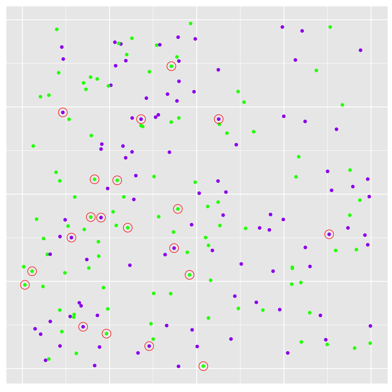
Figure 7.1: Plants sampled on the second occasion

This time we ended up sampling 11 green plants and 9 purple plants, so our second estimate of the purple morph frequency is 45%. This is quite different from the first estimate. It is actually lower than that seen in the original study population. Our hypothesis that the purple morph is more prevalent in the new population is beginning to look a little shaky in light of this second sample.

Nothing about the study population changed between the first and second sample. What’s more, we used a completely reliable sampling scheme to generate these samples—there was nothing biased or ‘incorrect’ about the way individuals were sampled. The two different estimates of purple morph frequency arise from nothing more than chance variation in the sampling process.

This variation–present whenever we observe a sample—has a special name. It is called sampling error. The word ‘error’ has nothing to do with mistakes or problems. In statistics, it is often used to refer to the variability or ‘noise’ in some process. Sampling error is the reason why we have to use statistics. Every time we estimate something there’s some sampling error lurking in the estimate. If we ignore it, we risk drawing incorrect conclusions about the world.

(By the way, another name for sampling error is ‘sampling variation.’ We’ll use both terms in this book because they are both widely used)

It is important to realise that sampling error is not really a property of any particular sample. It is a consequence of the nature of the variable(s) we’re studying and the sampling method used to investigate the population. Let’s try to understand what all this means.

7.2 Sampling distributions

We can develop our simple simulation example to explore the consequences of sampling error. This time, rather than taking one sample at a time, we will simulate thousands of independent samples. The number of plants sampled (‘n’) will always be 20. Every sample will be drawn from the same population, i.e. the population parameter (purple morph frequency) will never change across samples. This means any variation we observe is due to nothing more than sampling error.

Here is a graphical summary of one such repeated simulation exercise:

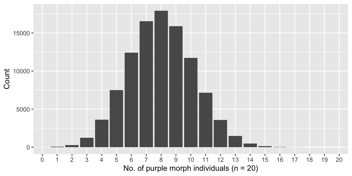
Figure 7.2: Distribution of number of purple morphs sampled (n = 20)

This bar plot summarises the results from taking 100000 independent samples of our population. Each time we took 20 individuals from our hypothetical population and calculated the number of purple morphs found. The bar plot shows the number of times we found 0, 1, 2, 3, … purple individuals, all the way up to the maximum possible (20). We could have converted these numbers to frequencies but we’re just summarising the raw distribution of purple morph counts at this point.

This distribution has a special name. It is called a sampling distribution. In order to work this out, we have to postulate values for the population parameters and we have to know how the population was sampled. This can often be done using mathematical reasoning. Here, we used brute-force simulation to approximate the sampling distribution of purple morph counts that arises when we sample 20 individuals from our hypothetical population.

What does this particular sampling distribution show? It shows us the range of outcomes we can expect to observe when we repeat the same sampling process over and over again. The most common outcome is 8 purple morphs, which would yield an estimate of 8/20 = 40% for the purple morph frequency.

Although there is no way to know this without being told, a 40% purple morph frequency is actually the number used to simulate the original, hypothetical data set. So it turns out that the true value of the parameter we’re trying to learn about also happens to be the most common estimate we expect to see under repeated sampling. That’s probably not too surprising.

Returning to our question—what is the purple morph frequency—we now have our answer. The purple morph frequency is 40%. Ok, but we have obviously ‘cheated’ here because we used information from 1000s of samples to arrive at that answer. In the real world we typically have to work with only one sample.

So what use is this sampling distribution idea? It turns out that sampling distributions are key to ‘doing frequentist statistics.’ To understand why we need to look a bit more carefully at that sampling distribution we made.

Look at the spread of the sampling distribution along the x-axis. The range of outcomes is roughly 2 to 15. This corresponds to estimated purple morph frequencies the in the range of 10-75%. This tells us that when we sample 20 individuals, the sampling error for a frequency estimate can be quite large.

The sampling distribution we summarised above is only relevant for the case where 20 individuals are sampled, and the frequency of purple plants in the population is 40%. If we change either of those two numbers and repeat the repeated sampling process we will end up with a different sampling distribution. That’s what was meant by, “It is a consequence of the nature of the variable(s) we’re studying and the sampling method used to investigate the population.”

Once we know how to calculate the sampling distribution for a particular problem, we can start to make statements about sampling error, to quantify uncertainty, and begin to address scientific questions. Fortunately, we don’t have to work any of the details out for ourselves—statisticians have already done the hard work for us.

7.3 The effect of sample size

One of the most important aspects of a sampling scheme is the sample size —often denoted ‘n.’ This is the number of observations of objects, items, etc in a sample. What happens when we change the sample size?

To get a sense of why sample size matters, we’ll repeat in our sampling exercise using two new sample sizes. First we’ll use a sample size of 40 individuals, then we’ll take a sample of 80 individuals. As before, we’ll take a total 100000 repeated samples from the population.

Here’s a graphical summary of the resulting sampling distributions:

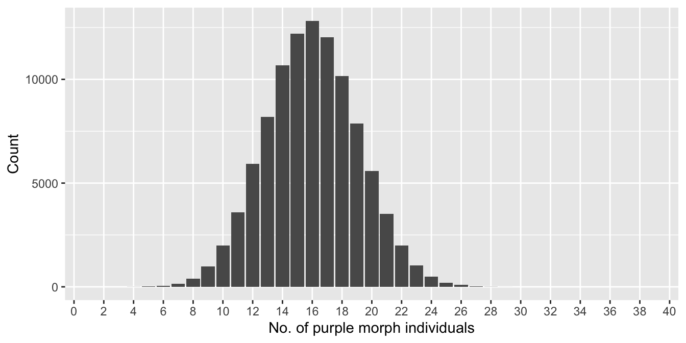
Figure 7.3: Distribution of number of purple morphs sampled (n = 40)

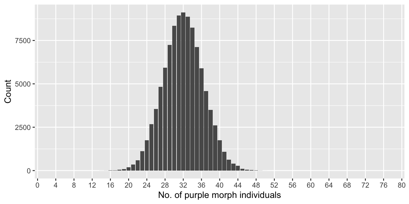
Figure 7.4: Distribution of number of purple morphs sampled (n = 80)

We plotted each of them over the full range of possible outcomes, i.e. the x axis runs from 0-40 and 0-80, respectively, in both plots. This is important because it allows us to compare the spread of each sampling distribution relative to the range of all possible outcomes. What do these two plots tell us about the effect of changing sample size?

The range of outcomes in the first plot (n = 40) is roughly 6 to 26, which corresponds to estimated purple morph frequencies in the range of 15-65%. The range of outcomes in the second plot (n = 80) is roughly 16 to 48, which corresponds to estimated frequencies in the range of 20-60%. The implications of this not-so-rigorous assessment are clear. We reduced sampling error by increasing the sample size. This makes intuitive sense: the composition of a large sample should more closely approximate that of the true population than a small sample.

How much data do we need to collect to accurately estimate a frequency? Here is the approximate sampling distribution of the purple morph frequency estimate when we sample 500 individuals:

## Warning: Removed 2 rows containing missing values (geom_bar).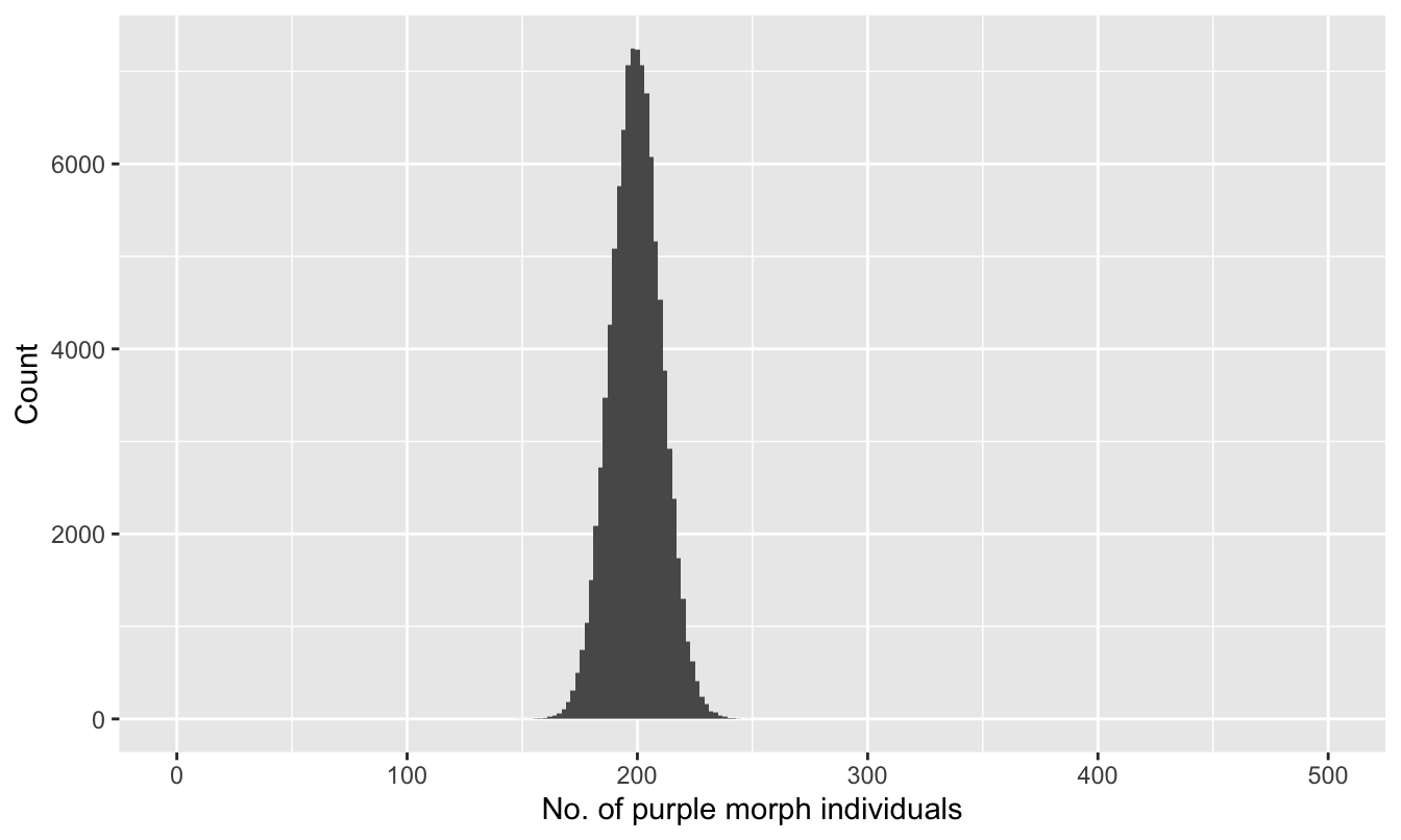

Figure 7.5: Distribution of number of purple morphs sampled (n = 500)

Now the range of outcomes is about 160 to 240, corresponding to purple morph frequencies in the 32-48% range. This is a big improvement over the smaller samples we just considered, but still, even with 500 individuals in a sample, we still expect quite a lot of uncertainty in our estimate. The take home message is that we need a lot of data to reduce sampling error.

7.4 The standard error

We’ve not been very careful about how we quantify the spread of a sampling distribution so far—we just estimated the range of purple morph counts by looking at histograms. This is fine for an investigation of general patterns, but to make rigorous comparisons, we really need a quantitative measure of sampling error variation. One such quantity is called the standard error.

The standard error is quite a simple idea, though its definition is a bit of mouthful: the standard error of an estimate is the standard deviation of the estimate’s sampling distribution. Don’t worry if that is confusing. Most of us find the definition of standard error confusing when we first encounter it. The key point is that it is a measure of the spread, or dispersion, of a distribution. The distribution in this case is the sampling distribution associated with some kind of estimate.

(It is common to use a shorthand abbreviations such “SE,” “S.E.” “se” or “s.e.” in place of ‘standard error’ when referring to the standard error in text.)

It’s much easier to make sense of something abstract like a standard error by looking at a concrete example. Let’s calculate the standard error of the estimated purple morph frequency. It is possible to do this using mathematical reasoning; however, it is much easier to understand what’s happening if we use ‘brute force’ simulations in R.

We’ll show you the code to as we go but keep in mind there’s really no need to commit any of it to memory. It’s just here for readers who like to see how things work. We start by specifying the number of samples to take (n_samples), the sample size to use for each sample (sample_size), and the value of the population morph frequency (purple_prob). We set up the simulation by creating these variables:

# number of independent samples
n_samples <- 100000
# sample size to use for each sample
sample_size <- 80
# probability a plant will be purple
purple_prob <- 0.4

This sets up a simulation to calculate the expected standard error when the purple morph frequency is 40% and the sample size is 80, using 10^{5} samples. The next step requires a bit more knowledge of R and probability theory:

# repeat the sampling/estimation procedure many times
raw_samples <- rbinom(n = n_samples, size = sample_size, prob = purple_prob)
# convert results to %
percent_samples <- 100 * raw_samples / sample_size

The details of the R code are not important here. A minimum of A-level statistics is needed to understand what the rbinom function is doing, but in a nutshell, it is the workhorse that runs the simulation. Mostly, we’re showing the code to demonstrate that seemingly complex things are often easy to do in R.

What matters here is the result. This is stored the result in a vector called percent_samples. Here are its first 50 values:

##  [1] 33.75 35.00 42.50 41.25 46.25 35.00 42.50 45.00 43.75 40.00 41.25 52.50
## [13] 43.75 38.75 38.75 47.50 42.50 40.00 43.75 42.50 36.25 42.50 43.75 43.75
## [25] 35.00 42.50 35.00 37.50 41.25 40.00 45.00 40.00 41.25 38.75 46.25 45.00
## [37] 31.25 40.00 47.50 42.50 37.50 41.25 31.25 45.00 32.50 36.25 40.00 37.50
## [49] 40.00 45.00

These numbers are all part of the sampling distribution of morph frequency estimates. Each value is one possible estimate of the purple morph frequency when we samples of 80 individuals from a population where the true value is 40%. There are 10^{5} such estimates stored in percent_samples.

How do we then calculate the standard error? This is defined as the standard deviation of the sampling distribution, which we just approximated with our simulation. So all we need to do now is calculate their standard deviation using the sd function:

sd(percent_samples)

## [1] 5.494663

The standard error is about 5.5. Why is this number useful? It gives us a means to reason about the variability in a sampling distribution. When a sampling distribution is ‘well-behaved,’ then roughly speaking, about 95% of estimates are expected to lie within a range of about four standard errors.

Not convinced? Look at the second bar plot we produced where the sample size was 80 and the purple morph frequency was 40%. What is the approximate range of simulated values? How close is this to \(4 \times 5.5\)? Quite close!

In summary, the standard error quantifies the variability of a sampling distribution. We said in the previous chapter that a point estimate is useless without some kind of associated measure of uncertainty. The standard error is one such measure.

7.5 What is the point of all this?

Why have we just spent so much time looking at what happens when we take repeated samples from a population with known properties? When we collect data in the real world we only have the luxury of working with a small number of samples—usually just one in fact. We also won’t know anything much the population parameter of interest in that situation. This lack of knowledge is the reason for collecting some data in the first place!

The short answer is that before we can use frequentist statistics we need to have a sense of:

• how point estimates behave under repeated sampling (i.e. sampling distributions),

• and how sampling error and standard error relate to sampling distributions.

Once we understand those ideas we’re can make sense of how frequentist statistical tests work. That’s what we’ll do in the next few chapters.