Chapter 6 Learning from data
Statistics is the science of learning from data, and of measuring, controlling, and communicating uncertainty; and it thereby provides the navigation essential for controlling the course of scientific and societal advances
The particular flavour of statistics covered in this book is called frequentist statistics. From a practical perspective, it is perfectly possible to apply frequentist tools by just learning a few basic ‘rules’ about how they work. That said, it is always easier to apply an technique if we understand at least roughly how it works.
The goal of the next few chapters is to provide an overview of some core frequentist concepts. We are not going to cover the underpinning mathematics! Instead, we aim to arrive at a conceptual feel for the important underpinning ideas. These are difficult to understand at first. This is fine. We’ll return to them over and over again as we introduce different statistical models and tests.
We’re going to start by laying out a somewhat simplified overview of the steps involved in ‘doing frequentist statistics’ in this chapter. We’ll also introduce some few key definitions along the way. Later chapters will then drill into the really important concepts—things like sampling variation, standard errors, null hypotheses and p-values.
6.1 Populations
When a biologist talks about a population they usually mean a group of individuals of the same species who interact. What does a statistician mean when they talk about populations? The word has a very different meaning in statistics. Indeed, it is a much more abstract concept: a statistical population is any group of items or objects that share certain attributes or properties.
This is best understood by example…
The readers of this book could be viewed as a statistical population. This book is targeted at undergraduate students with an interest in biology. That group are mostly in their late teens and early 20s, and they tend to have similar educational backgrounds and career aspirations. As a consequence of these similarities, these students tend to be more similar to one another than they would be to a randomly chosen inhabitant of say, the US or Germany.
The different areas of peatland in the UK can be thought of as a statistical population. There are many peatland sites in the UK, and although their precise ecology varies from one location to the next, they are also very similar in many respects. Peatland habitat is generally characterised by low-growing vegetation and acidic soils. If you visit two different peatland sites in the UK, they will seem quite similar compared to, for example, a neighbouring calcareous grassland.
A population of plants or animals (as typically understood by biologists) can also be thought of as a statistical population. Indeed, this is often the kind of population ecologists are interested in. The individuals that comprise a biological population share common behaviours and physiology characteristics. Much of organismal biology is concerned with learning about these properties of organisms.
Populations are conceptualised as fixed but essentially unknown entities within the framework of frequentist statistics. The goal of statistics is to learn something about populations by analysing data collected from them. It is important to realise that ‘the population’ is defined by the investigator, and the ‘something we want to learn about’ can be anything we know how to measure.
Consider the examples again:
A social scientist might be interested in the political attitudes of undergraduates, so they choose to survey a group of students at university.
A climate change scientist might measure the mass of carbon that is stored in peatland areas at sites across Scotland and northern England.
A behavioural ecologist might want to understand how much time beavers spend foraging for food, so they might study a Scottish population.
OK, so how does the process of learning about a population from data actually work?
6.2 Learning about populations
The examples discussed above involve very different kinds of populations, questions and data. Nonetheless, there are fundamental commonalities in how those questions could be addressed. The process can be broken down into a number of distinct steps:
Step 1: Refine your questions, hypotheses and predictions
This step was discussed in scientific process chapter. The key point is that we should never begin collecting data until we’ve set out the relevant questions, hypotheses and predictions. This might seem obvious, but it is surprising how often people don’t get these things straight before diving into data collection. Collecting data without a clear scientific objective and rationale is guaranteed to waste a lot of time and energy.
Step 2: Decide which population(s) is (are) important
The second step is to decide which population(s) we should study. What constitutes ‘the population’ will be fairly obvious in some kinds of study. In the three cases considered above, the corresponding populations we choose to study could be undergraduate students at a university, peatland habitats from across the UK, and beavers in Scotland. In all three examples it was fairly easy to define what we mean by ‘a population’ (though that doesn’t mean the populations are easy to study—we’ll return to this idea later).
The problem of deciding which population(s) to study can be more subtle than it first appears. What happens if we’re planning an experiment? Imagine that we want to test a prediction that nutrient addition reduces biodiversity in chalk grasslands. We might set up an experiment with two kinds of plots:
manipulated plots where we add fertiliser, and
control plots where we do nothing.
Comparing these in some way would allow us to assess the impact of adding nutrients. That’s easy enough to understand.
What can we say about the statistical populations in this example? First, there are two of them, control and manipulated communities, and these two populations are completely defined by the experimental design. The nutrient addition plots don’t ‘exist’ until we do the experiment. That’s not hugely intuitive. What’s more, the weird mental contortion that a frequentist does is to imagine that the experimental plots are part of some larger, unobserved population of nutrient addition plots.
The important point is that statistical populations are something the investigator defines. They might be ‘real,’ undergraduates at university, or they might be something that doesn’t really exist in a meaningful way, like a population of not-yet-realised experimentally manipulated plots. In either case, we can use the same statistical techniques to learn something general about ‘the population(s).’
Step 3: Decide which variables to study
The next step is to decide which attributes of the items that comprise our population(s) need to be measured. This comes down to deciding which variable(s) to measure. We discussed some of the considerations in the data and variables chapter. In the examples above, the appropriate variables would be things like a standardised measure of political attitude, the mass of stored carbon per unit area, or the body mass of individuals.
This step is often straightforward, though some effort may be required to pick among different options. There isn’t a whole lot of ambiguity associated with a physical variable like body mass, but something like ‘political attitude’ needs careful thought. Can we quantify this by studying just one thing, like voting patterns? Probably not. Maybe we need to measure several things and aggregate those in some way.
Step 4: Decide which population parameters are relevant
Once we have decided which variables to study, we have to decide which population parameters are relevant. A population parameter is simple a numeric quantity that describes the variable(s) we want to learn about. A population parameter describes a property of that variable in the population. It’s not a property of our actual data.
A simple population parameter familiar to many people is the population mean. We often study means because they allows us to answer questions like, “how much, on average, of something is present?” Quite a number of the statistical tests in this book biol down to asking questions of population means. That doesn’t mean we can’t ask questions about other kinds of population parameters:
Statistical genetics aims to partition variability among individuals—we want to know how much phenotypic variation is due to genetic vs. non-genetic sources. In this case it is population variances we want to learn about.
Sometimes we want to understand how two or more aspects of the population are associated with one another. In this situation a correlation coefficient might be the right population parameter to focus on.
Once we have identified the population parameter we care about we need a way to learn something about it. That takes us to the next step.
Step 5: Gather a representative sample
We wouldn’t need statistics if we could measure every member of a population because we could simply calculate the parameter of interest from an exhaustive sample. However, in the real world we have limited time and money to invest in any problem, no matter how important. This means we have to work with an more limited sample of the population.
A sample is a subset of a population that has been selected to be representative. That word ‘representative’ is really important in this context. A representative sample one that reflects the characteristics of the entire population. It is really important to use sampling methods that lead to representative samples.
Why? Put simply, it’s hard to infer anything useful about a population from non-representative sample. For example, if we aim to understand the reproductive characteristics of our favourite study organism, but we only sample old-aged individuals, it will be impossible to generalise our findings when reproductive performance changes with age.
Collecting larger samples does not solve this kind of problem. For example, a sample that contains every single old-age individual but few younger individuals still doesn’t tell us much about the younger age group. People often assume that ‘more data = better data’ but that isn’t be true if those data are not representative of the population they actually care about. Try to remember that in your own work.
The study of how to gather useful samples from populations and use these calculate meaningful estimates is an important part of statistics. It falls under the banners of experimental design and sampling theory. These are large, technical topics that are well beyond the scope of this book. However, we will touch on a few of the more important practical aspects in later chapters.
Step 6: Estimate the population parameter
After we have acquired a representative sample from a population we can calculate something called a point estimate of the population parameter. Remember, that parameter is ultimately unknown. A point estimate is a number that represents our ‘best guess’ at its true, unknown value. For example, if we are interested in the population mean, the obvious point estimate to use is the ‘the average’ we learn about at school.
There are many different kinds of point estimates we can calculate. What we choose to estimate depends of the question we’re answering. If we care about variability we might calculate one or more sample ‘variances.’ Sometimes we have to calculate some kind of aggregate measure of an effect, like the difference between two sample means.
(By the way, people often say ‘estimate’ instead of ‘point estimate,’ for the simple reason that saying or writing ‘point estimate’ all the time soon becomes tedious. We use both terms in this book.)
Step 7: Estimate uncertainty
A point estimate is fairly useless on its own. Why? Because it is derived from a limited sample of the population. Even if we collect a really large representative sample, its composition won’t exactly match that of the population. This means any point estimate we derive from the sample will be imperfect, in that it won’t exactly match the true population value.
There is always some uncertainty associated with estimates population parameters. Our job as scientists is to to find a way to quantify that uncertainty. This part of the frequentist method is probably the hardest to understand so we’ll spend a fair bit of time thinking about it later in the sampling error chapter.
Step 8: Answer the question!
Once we have our point estimates and measures of uncertainty we’re finally in the position to start answering questions.
Imagine that we want to answer a seemingly simple question, e.g. “Are there more than 200 tonnes of carbon per hectare stored in the peatland of the Peak District?” We might sample a number of sites, measure the stored carbon at each of these, and then calculate the mean of these measurements. What should we conclude if the sample mean is 210 t h-1? We can’t say much until we have a sense of how reliable that mean is likely to be. To answer our question, we have to know how to assess whether or not the difference we observe (210 - 200 = 10) was just a fluke.
The tools we’ll learn about in this book are designed to answer a range of different kinds of scientific question. Nonetheless, they all boil down to the same basic question: Is the pattern I see ‘real,’ or is it instead likely to be a result of chance variation? To tackle this, we combine point estimates and measures of uncertainty in various ways. Statistical software like R will do the hard work for us, but we still just have to learn how to interpret the results it gives us.
6.3 A simple example
The best way to get a sense of how all this fits together is by working through an example. We’ll finish this chapter by introducing a very simple example. It is worth paying attention to this as we’ll use again in later chapters. We’re going to work through steps 1-6 here. The final two steps are sufficiently challenging that they need their own chapters.
Imagine we’re interested in a plant species that is phenotypically polymorphic. There are two different ‘morphs,’ a purple morph and a green morph. We can depict this situation visually with a map showing where purple and green plants are located on a hypothetical landscape:
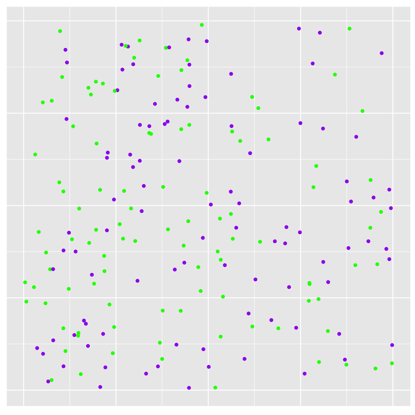
Figure 6.1: Stylised landscape showing a population of purple and green plants
These are idealised data generated using a simulation in R. Let’s proceed as though these are real data…
Step 1: Refine your questions, hypotheses and predictions
Imagine we had also previously studied a different population of this species that exhibits the same polymorphism. We’re fairly sure both populations were once connected. However, habitat loss over has significantly reduced the connectance between them.
Our previous studies with the old neighbouring population have shown:
The colour polymorphism is controlled by a single gene with two alleles: a recessive mutant allele (‘P’) confers the purple colour and the dominant wild-type allele (‘G’) makes plants green. Genetic work has shown that the two alleles are present in a ratio of about 1:1 in the neighbouring population.
There seems to be no observable fitness difference between the two morphs in the neighbouring population. What’s more, about 25% of plants are purple. This suggests that the two alleles are in Hardy-Weinberg equilibrium. These observations suggest that there is no selection operating on the polymorphism.
Things are different in the new study population. The purple morph seems to be about as common as the green morph, and preliminary research indicates purple plants seem to produce more seeds than green plants. Our hypothesis is, therefore, that purple plants have a fitness advantage in the new study population. A prediction that follows from this is that the frequency of the purple morph will be greater than 25% in the new study population, as selection is driving the ‘P’ allele to fixation.
(This isn’t the strongest test of our hypothesis, by the way. Really, we need to study allele and genotype frequencies, not just phenotypes. It is good enough for illustrative purposes.)
Step 2: Decide which population is important
This situation is entirely made up, so consideration of the statistical population is a little artificial. In the real world, we would consider various factors, such as whether or not we can study the whole population or must restrict ourselves to one sub-population. Working at a large scale should produce a more general result, but it could also present a significant logistical challenge.
Step 3: Decide which variables to study
This step is easy. We could measure all kinds of different attributes of the plants—biomass, height, seed production, etc—but to study the polymorphism we only need to collect information about the colour of different individuals. This means we are going to be working with a nominal variable that takes two values: ‘purple’ or ‘green.’
Step 4: Decide which population parameters are relevant
The prediction we want to test is about the purple morph frequency, or equivalently, the percentage, or proportion, of purple plants. Therefore, the relevant population parameter is the frequency of purple morphs in the wider population. We need to collect data that would allow us learn about this unknown quantity.
Step 5: Gather a representative sample
A representative sample in tis situation is one in which every individual on the landscape has the same probability of being sampled. This is what people actually mean when they refer to a ‘random sample.’ Gathering a random sample of organisms from across a landscape is surprisingly hard to do. Fortunately, it is very easy to do in a simulation. Let’s seen what happens if we sample 20 plants at random…
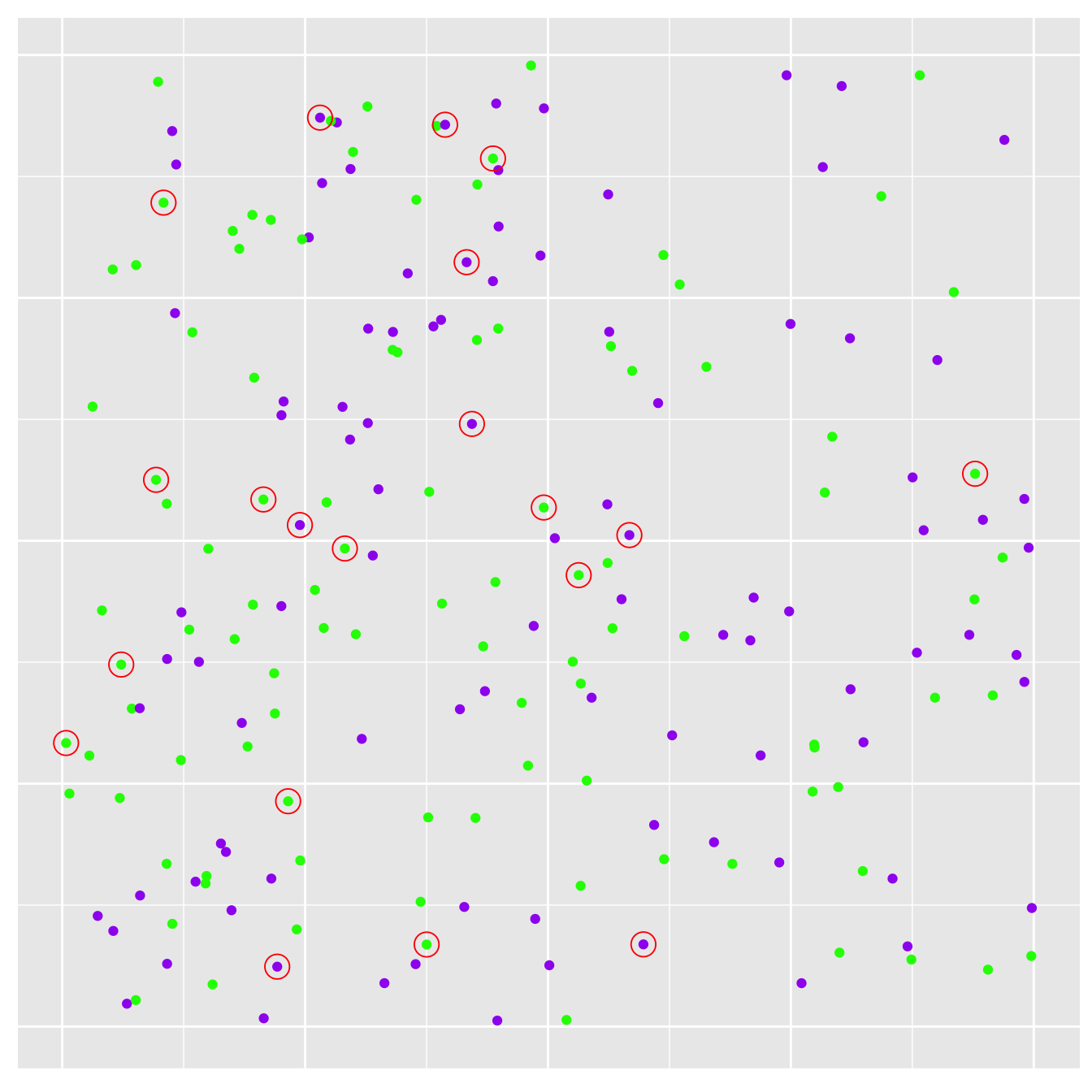
Figure 6.2: Sampling plants. Sampled plants are circled in red
The new plot shows the original population of plants, only this time we’ve circled the sampled individuals in red.
Step 6: Estimate the population parameter
Estimating a frequency from a sample is simple enough though we can express frequencies in different ways. We’ll use a percentage. We found 12 green plants and 8 purple plants in our sample, which means our point estimate of the purple morph frequency is 40%. This is certainly greater than 25%—the value of observed in the original population—but it isn’t that far off if you consider that this is from quiet a small sample.
6.4 Now what?
Maybe the purple plants aren’t at a selective advantage after all? Or perhaps they are? We’ll need to develop a rigorous statistical test of some kind to evaluate our prediction. Before we can do this we need to delve into a few more concepts. The first of these, sampling error, is needed describe the uncertainty in the purple morph frequency estimate (step 7). We’ll look at this topic in the next chapter. After that, we’ll be in the position to answer our question about differences among the two populations (step 8).