Chapter 13 Two-sample t-test
13.1 When do we use a two-sample t-test?
The two-sample t-test is a parametric version of the permutation procedure we studied in the statistical comparisons chapter. The test can be used to compare the means of a numeric variable sampled from two independent populations. The aim of a two-sample t-test is to evaluate whether or not the mean is different in the two populations. Here are two examples:
We’re studying how the dietary habits of Scandinavian eagle-owls vary among seasons. We suspect that the dietary value of a prey item is different in the winter and summer. To evaluate this prediction, we measure the size of Norway rat skulls in the pellets of eagle-owls in summer and winter, and then compare the mean size of rat skulls in each season using a two-sample t-test.
We’re interested in the costs of anti-predator behaviour in Daphnia spp. We conducted an experiment where we added predator kairomones—chemicals that signal the presence of a predator—to jars containing individual Daphnia. There is a second control group where no kairomone was added. The change in body size of individuals was measured after one week. We could use a two-sample t-test to compare the mean growth rate in the control and treatment groups.
13.2 How does the two-sample t-test work?
Imagine we have taken a sample of a variable from two populations, labelled ‘A’ and ‘B.’ We’ll call the variable ‘X’ again. Here’s an example of how these kinds of data might look if we had a sample of 50 items from each population:
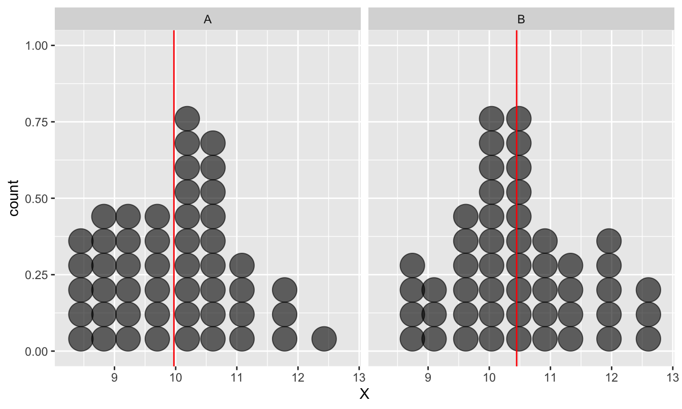
Figure 13.1: Example of data used in a two-sample t-test
The first thing to notice is the two distributions overlap quite a lot. However, this observation isn’t necessarily all that significant. Why? Because we’re not interested in the raw values of ‘X’ in the two samples. It’s the difference between the means that our test is going to focus on.
The red lines show the mean of each sample. Sample B obviously has a larger mean than sample A. The question is, how do we decide whether this difference is ‘real,’ or purely a result of sampling variation?
Using a frequentist approach, we tackle this question by first setting up the appropriate null hypothesis. The null hypothesis here is one of no difference between the population means (they are equal). We then have to work out what the null distribution looks like. This is sampling distribution of the difference between sample means under the null hypothesis. Once we have the null distribution worked out we can calculate a p-value.
How is this different from the permutation test? The logic is virtually identical. The one important difference is that we have to make an extra assumption to use the two-sample t-test. We assume the variable is normally distributed in each population. If this assumption is valid, then the null distribution will have a known form—a t-distribution.
We only need a few pieces of information to carry out a two-sample t-test. These are basically the same quantities needed to construct the one-sample t-test, except now there are two samples involved. We need the sample sizes of groups A and B, the sample variances and the estimated difference between the sample means of X in A and B.
How does two-sample t-test actually work? It is carried out as follows:
Step 1. Calculate the two sample means then calculate the difference between these estimates. This estimate is our ‘best guess’ of the true difference between means. As with the one-sample test, its role in the two-sample t-test is to allow us to construct a test statistic.
Step 2. Estimate the standard error of the difference between the sample means under the null hypothesis of no difference. This gives us an idea of how much sampling variation we expect to observe in the estimated difference, if there were actually no difference between the means.
There are a number of different options for estimating this standard error. Each one makes a different assumption about the variability of the two populations. Which ever choice we make the calculation always boils down to a simple formula involving the sample sizes and sample variances. The standard error gets smaller when the sample sizes grow, or when the sample variances shrink. That’s the only important point, really.
Step 3. Once we have estimated the difference between sample means and its standard error, we can calculate the test statistic. This is a type of t-statistic, which we calculate by dividing the difference between sample means (from step 1) by the estimated standard error of the difference (from step 2):
\[\text{t} = \frac{\text{Difference Between Sample Means}}{\text{Standard Error of the Difference}}\]
This t-statistic is guaranteed to follow a t-distribution if the normality assumption is met. This knowledge leads to the final step…
Step 4. Compare the test statistic to the theoretical predictions of the t-distribution to assess the statistical significance of the observed difference. That is, we calculate the probability that we would have observed a difference between means with a magnitude as large as, or larger than, the observed difference, if the null hypothesis were true. That’s the p-value for the test.
We willnot step through the various calculations involved in these steps. The formula for the standard two-sample t-test and its variants are summarised on the t-test Wikipedia page. There’s absolutely no need to learn these because we’re going to let R to handle the calculations for us.
Let’s review the assumptions of the two-sample t-test first…
13.2.1 Assumptions of the two-sample t-test
Several assumptions need to be met for a two-sample t-test to be valid. These are basically the same as those for the one-sample version. Starting with the most important and working down in decreasing order of importance, these are:
Independence. Remember what we said in our discussion of the one-sample t-test? If the data are not independent, the p-values generated by the test will be too small, and even mild non-independence can be a serious problem. The same is true of the two-sample t-test.
Measurement scale. The variable we are working with should be measured on an interval or ratio scale, which means it will be numeric. It makes little sense to apply a two-sample t-test to a categorical variable of some kind.
Normality. The two-sample t-test will produce reliable p-values if the variable is normally distributed in each population. However, the two-sample t-test is fairly robust to mild departures from normality and this assumption matters little when the sample sizes are large.
13.2.2 Evaluating the assumptions
How do we evaluate the first two assumptions? As with the one-sample test, these are aspects of experimental design—we can only evaluate them by thinking about the data we’ve collected.
The normality assumption can be evaluated by plotting the the sample distribution of each group using, for example, a pair of histograms or dot plots. We must examine the distribution in each group, not the distribution of the combined sample. If both samples looks approximately normal then we can proceed with the test. If we think we can see a departure from normality then we should consider our sample sizes before deciding to proceed, remembering that the test is robust to mild departures when sample sizes are large (e.g. >100 observations in each group).
13.2.3 What about the equal variance assumption?
It is sometimes said that a two-sample t-test requires the variability (‘variance’) of each sample to be the same, or at least quite similar. This would be true if we used the original version of Student’s two-sample t-test. However, R doesn’t use this version of the test by default. R uses the “Welch” two-sample t-test. This version of the test does not rely on the equal variance assumption. As long as we stick with this version of the t-test, the equal variance assumption isn’t something we need to worry about.
Should we use Student’s original two-sample t-test?
The original ‘equal-variance’ two-sample t-test is a little more powerful than the Welch version; that is, it is more likely to detect a difference in means (if present). However, the increase in statistical power is really quite small if the sample sizes of each group are similar and the original test is only correct when the population variances are identical. Since we can never prove the ‘equal variance’ assumption—we can only ever reject it—it is generally safer to just use the Welch two-sample t-test.
One last warning. Student’s two-sample t-test assumes the variances of the populations are identical. It is the population variances, not the sample variances, that matter. There are methods for comparing variances, and people sometimes suggest using these to select ‘the right’ t-test. This is bad advice. For reasons just outlined, there’s little advantage to using Student’s version of the test if the variances really are the same. What’s more, the process of picking the test based on the results of another statistical test affects the reliability of the resulting p-values.
13.3 Carrying out a two-sample t-test in R
##
## ── Column specification ────────────────────────────────────────────────────────
## cols(
##   Colour = col_character(),
##   Weight = col_double()
## )
Work through the example in this section. We’re going to use the plant morph example one last time. Everything below assumes ‘MORPH_DATA.CSV’ has been read into an R data frame called morph_data.
We’ll use with the plant morph size example again to learn the work flow for two-sample t-tests in R. We’ll use the test to evaluate whether or not the mean dry weight of purple plants is different from that of green plants. The background to why this comparison is worth doing was covered in the statistical comparisons chapter. We considered this comparison using a permutation test in that chapter. It’s actually much simpler to use a two-sample t-test, as we are about to find out…
13.3.1 Visualising the data and checking the assumptions
We start by calculating a few descriptive statistics and visualising the sample distributions of the green and purple morph dry weights. We already did this in the statistical comparisons chapter but here’s the dplyr code for the descriptive statistics again:
morph_data %>%
  # group the data by plant morph
  group_by(Colour) %>%
  # calculate the mean, standard deviation and sample size
  summarise(mean = mean(Weight),
            sd = sd(Weight),
            samp_size = n())
## `summarise()` ungrouping output (override with `.groups` argument)## # A tibble: 2 x 4
## Colour mean sd samp_size
## <chr> <dbl> <dbl> <int>
## 1 Green 708. 150. 173
## 2 Purple 767. 156. 77As we already know the purple plants tend to be a bigger than green plants. The sample sizes are 173 (green plants) and 77 (purple plants). These are good-sized samples, which means we probably don’t need to be too obsessed about the normality assumption. However, we still need to visualise the sample distributions to be sure they aren’t too odd or contain obvious outliers:
ggplot(morph_data, aes(x = Weight)) +
  geom_histogram(binwidth = 50) +
  facet_wrap(~Colour, ncol = 1)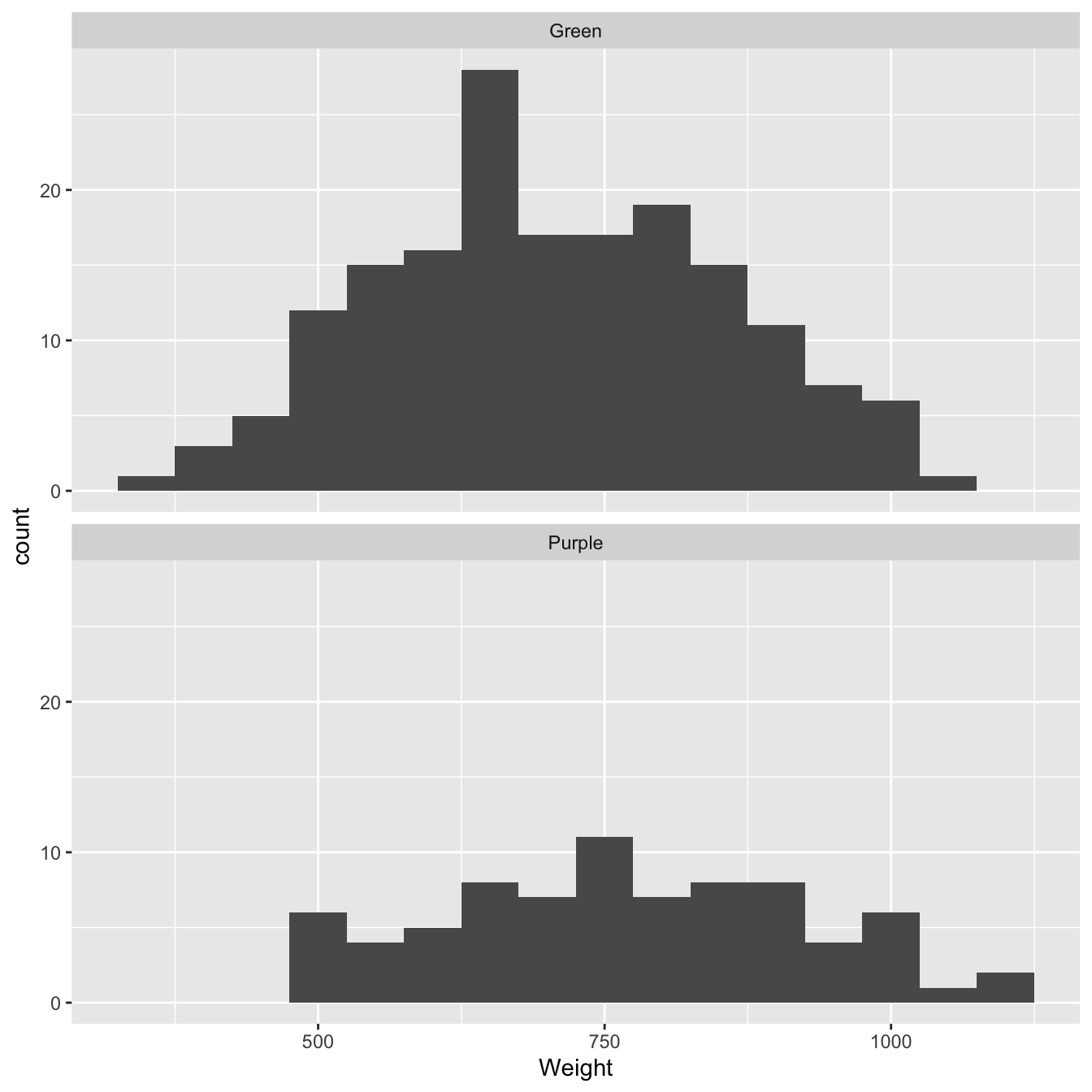
Figure 13.2: Size distributions of purple and green morph samples
There is nothing too ‘non-normal’ about the two samples in this example so it’s reasonable to assume they both came from normally distributed populations.
13.3.2 Carrying out the test
The function we need to carry out a two-sample t-test in R is the t.test function, i.e. exactly the same functions used for the one-sample test.
Remember, morph_data has two columns: Weight contains the dry weight biomass of each plant, and Colour is an index variable that indicates which sample (plant morph) an observation belongs to. Here’s the code to carry out the two-sample t-test:
t.test(Weight ~ Colour, morph_data)We suppressed the output for now to focus on how to use the function. We have to assign two arguments:
The first argument is something called a formula. We know this because it includes a ‘tilde’ symbol:
~. The variable name on the left of the~must be the variable whose mean we want to compare (Weight). The variable on the right must be the indicator variable that says which group each observation belongs to (Colour).The second argument is the name of the data frame that contains the variables listed in the formula.
Let’s take a look at the output:
t.test(Weight ~ Colour, morph_data)##
## Welch Two Sample t-test
##
## data: Weight by Colour
## t = -2.7808, df = 140.69, p-value = 0.006165
## alternative hypothesis: true difference in means is not equal to 0
## 95 percent confidence interval:
## -100.46812 -16.97476
## sample estimates:
## mean in group Green mean in group Purple
## 707.8424 766.5638The first line reminds us what kind of t-test we used. This says: Welch two-sample t-test, so we know that we used the Welch version of the test that accounts for the possibility of unequal variance. The next line reminds us about the data. This says: data: Weight by Colour, which is R-speak for ‘we compared the means of the Weight variable, where the group membership is defined by the values of the Colour variable.’
The third line of text is the most important. This says: t = -2.7808, d.f. = 140.69, p-value = 0.006165. The first part, t = -2.7808, is the test statistic (i.e. the value of the t-statistic). The second part, df = 140.69, summarise the ‘degrees of freedom’ (see the box below). The third part, p-value = 0.006165, is the all-important p-value. This says there is a statistically significant difference in the mean dry weight biomass of the two colour morphs, because p<0.05. Because the p-value is less than 0.01 but greater than 0.001, we would report this as ‘p < 0.01.’
The fourth line of text (alternative hypothesis: true difference in means is not equal to 0) simply reminds us of the alternative to the null hypothesis (H1). This isn’t hugely important or interesting.
The next two lines show us the ‘95% confidence interval’ for the difference between the means. Just as with the one sample t-test we can think of this interval as a rough summary of the likely values of the true difference (again, a confidence interval is more complicated than that in reality).
The last few lines summarise the sample means of each group. This could be useful if we had not bothered to calculate these already.
A bit more about degrees of freedom
In the original version of the two-sample t-test (the one that assumes equal variances) the degrees of freedom of the test are give by (nA-1) + (nB-1), where nA is the number of observations in sample A, and nB the number of observations in sample B. The plant morph data included 77 purple plants and 173 green plants, so if we had used the original version of the test we would have (77-1) + (173-1) = 248 d.f.
The Welch version of the t-test reduces the numbers of degrees of freedom by using a formula that takes into account the difference in variance in the two samples. The greater the difference in the two sample sizes the smaller the number of degrees of freedom becomes:
-
When the sample sizes are similar, the adjusted d.f. will be close to that in the original version of the two-sample t-test.
-
When the sample sizes are very different, the adjusted d.f. will be close to the sample size of the smallest sample.
Note that the ‘unequal sample size accounting’ results in degrees of freedom that are not whole numbers. It’s not critical that you remember all this. Here’s the important point: whatever flavour of t-test we’re using, a test with high degrees of freedom is more powerful than one with low degrees of freedom, i.e. the higher the degrees of freedom, the more likely we are to detect an effect if it is present. This is why degrees of freedom matter.
13.3.3 Summarising the result
Having obtained the result we need to report it. We should go back to the original question to do this. In our example the appropriate summary is:
Mean dry weight biomass of purple and green plants differs significantly (Welch’s t = 2.78, d.f. = 140.7, p < 0.01), with purple plants being the larger.
This is a concise and unambiguous statement in response to our initial question. The statement indicates not just the result of the statistical test, but also which of the mean values is the larger. Always indicate which mean is the largest. It is sometimes appropriate to also give the values of the means:
The mean dry weight biomass of purple plants (767 grams) is significantly greater than that of green plants (708 grams) (Welch’s t = 2.78, d.f. = 140.7, p < 0.01)
When we are writing scientific reports, the end result of any statistical test should be a statement like the one above—simply writing t = 2.78 or p < 0.01 is not an adequate conclusion!