Chapter 12 One sample t-tests

12.1 When do we use one-sample t-test?

The one-sample t-test is a very simple statistical test. It is used when we have a sample of numeric variable, and we want to compare its population mean to a particular value. The one-sample t-test evaluates whether the population mean is likely to be different from this value. The expected value could be any value we are interested in. Here are a couple of specific examples:

We have developed a theoretical model of foraging behaviour that predicts an animal should leave a food patch after 10 minutes. If we have data on the actual time spent by 25 animals observed foraging in the patch, we could test whether the mean foraging time is ‘significantly different’ from the prediction using a one-sample t-test.
We are monitoring sea pollution and have collected a series of water samples from a beach. We wish to test whether the mean density of faecal coliforms—bacteria indicative of sewage discharge—can be regarded as greater than the legislated limit. A one-sample t-test will test whether the mean value for the beach as a whole exceeds this limit.

Let’s see if we can get sense of how these tests would work.

12.2 How does the one-sample t-test work?

Imagine we have taken a sample of some variable and we want to evaluate whether its mean is different from some number (the ‘expected value’).

Here’s an example of what these data might look like if we had used a sample size of 50:

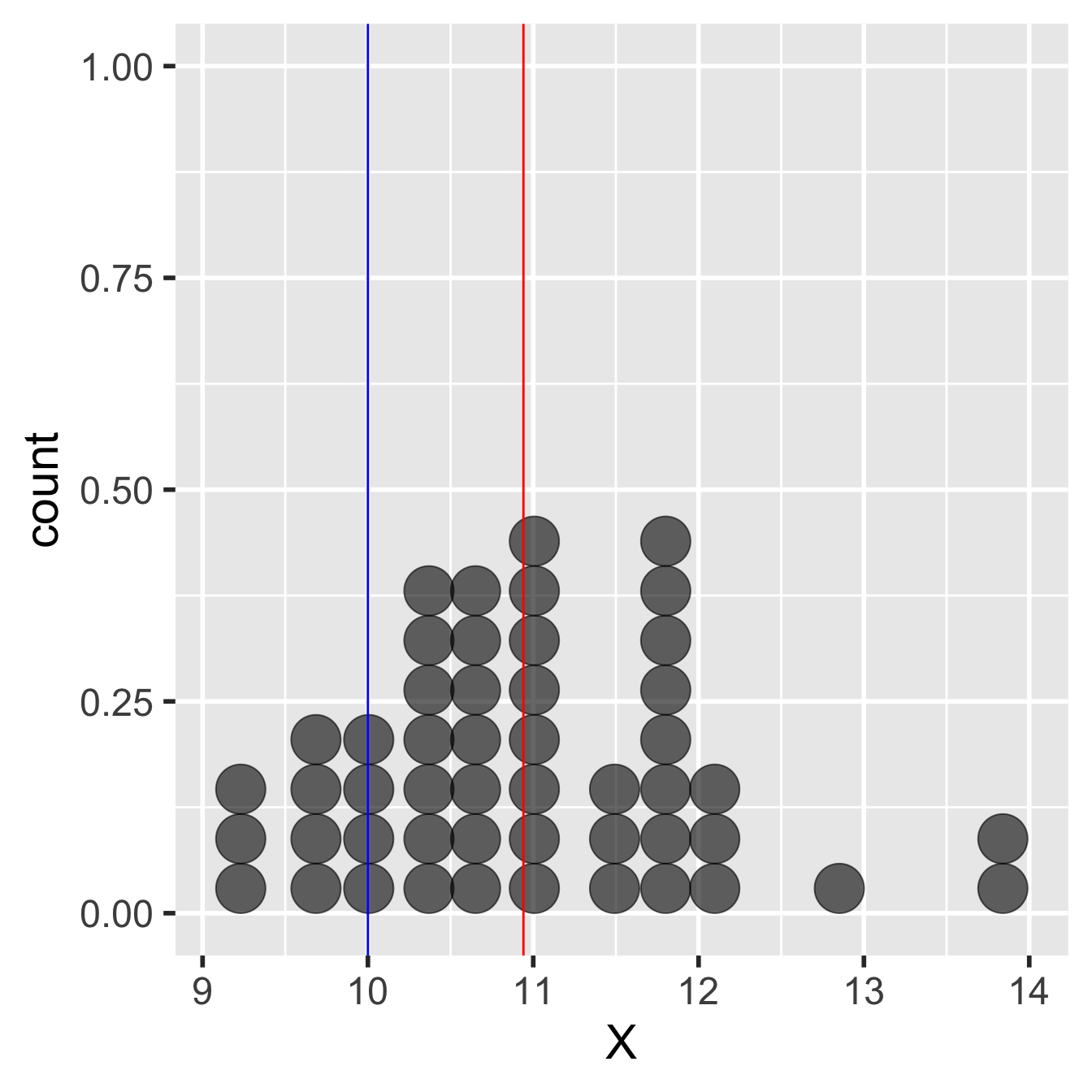
Figure 12.1: Example of data used in a one-sample t-test

We’re calling the variable ‘X’ in this example. It needs a label and ‘X’ is as good as any other. The red line shows the sample mean. This is a bit less than 11. The blue line shows the expected value. This is 10, so this example could correspond to the foraging study mentioned above.

The observed sample mean is about one unit larger than the expected value. The question is, how do we decide whether the population mean is really different from the expected value? Perhaps the difference between the observed and expected value is due to sampling variation. Here’s how a frequentist tackles this kind of question:

Set up an appropriate null hypothesis, i.e. an hypothesis of ‘no effect’ or ‘no difference.’ The null hypothesis in this type of question is that the population mean is equal to the expected value.
Work out what the sampling distribution of a sample mean looks like under the null hypothesis. This is the null distribution. Because we’re now using a parametric approach, we will assume this has a particular form.
Finally, we use the null distribution to assess how likely the observed result is under the null hypothesis. This is the p-value calculation that we use to summarise our test.

This chain of reasoning is no different from that developed in the bootstrapping example from earlier. We’re just going to make an extra assumption this time to allow us to use a one-sample t-test. This extra assumption is that the variable (‘X’) is normally distributed in the population. When we make this normality assumption the whole process of carrying out the statistical test is actually very simple because the null distribution will have a known mathematical form—it ends up being a t-distribution.

We can use this knowledge to construct the test of statistical significance. Instead of using the whole sample, as we did with the bootstrap, now we only need three simple pieces of information to construct the test: the sample size, the sample variance, and the sample mean. The one-sample t-test is then carried out as follows:

Step 1. Calculate the sample mean. This happens to be our ‘best guess’ of the unknown population mean. However, its role in the one-sample t-test is to allow us to construct a test statistic in the next step.

Step 2. Estimate the standard error of the sample mean. This gives us an idea of how much sampling variation we expect to observe. The standard error doesn’t depend on the true value of the mean, so the standard error of the sample mean is also the standard error of any mean under any particular null hypothesis.

This second step boils down to applying a simple formula involving the sample size and the standard deviation of the sample:

\[\text{Standard Error of the Mean} = \sqrt{\frac{s^2}{n}}\]

…where $s^2$ is the square of the standard deviation (the sample variance) and $n$ is for the sample size. This is the formula introduced in the parametric statistics chapter. The standard error of the mean gets smaller as the sample sizes grows or the sample variance shrinks.

Step 3. Calculate a ‘test statistic’ from the sample mean and standard error. We calculate this by dividing the sample mean (step 1) by its estimated standard error (step 2):

\[\text{t} = \frac{\text{Sample Mean}}{\text{Standard Error of the Mean}}\]

If our normality assumption is reasonable this test-statistic follows a t-distribution. This is guaranteed by the normality assumption. So this particular test statistic is also a t-statistic. That’s why we label it t. This knowledge leads to the final step…

Step 4. Compare the t-statistic to the theoretical predictions of the t-distribution to assess the statistical significance of the difference between observed and expected value. We calculate the probability that we would have observed a difference with a magnitude as large as, or larger than, the observed difference, if the null hypothesis were true. That’s the p-value for the test.

We could step through the actual calculations involved in these steps in detail, using R to help us, but there’s no need to do this. We can let R handle everything for us. But first, we should review the assumptions of the one-sample t-test.

12.2.1 Assumptions of the one-sample t-test

There are a number of assumptions that need to be met in order for a one-sample t-test to be valid. Some of these are more important than others. We’ll start with the most important and work down the list in reverse order of importance:

Independence. In rough terms, independence means each observation in the sample does not ‘depend on’ the others. We’ll discuss this more carefully when we consider the principles of experimental design. The key thing to know now is why this assumption matters: if the data are not independent the p-values generated by the one-sample t-test will be unreliable.

(In fact, the p-values will be too small when the non-independence assumption is broken. That means we risk the false conclusion that a difference is statistically significant, when in reality, it is not)

Measurement scale. The variable being analysed should be measured on an interval or ratio scale, i.e. it should be a numeric variable of some kind. It doesn’t make much sense to apply a one-sample t-test to a variable that isn’t measured on one of these scales.
Normality. The one-sample t-test will only produce completely reliable p-values when the variable is normally distributed in the population. However, this assumption is less important than many people think. The t-test is robust to mild departures from normality when the sample size is small, and when the sample size is large the normality assumption hardly matters at all.

We don’t have the time to explain why the normality assumption is not too important for large samples, but we can at least state the reason: it is a consequence of that central limit theorem we mentioned in the last chapter.

12.2.2 Evaluating the assumptions

The first two assumptions—independence and measurement scale—are really aspects of experimental design. We can only evaluate these by thinking carefully about how the data were gathered and what was measured. It’s too late to do anything about these after we have collected our data.

What about that 3^rd assumption—normality? One way to evaluate this is by visualising the sample distribution. For small samples, if the sample distribution looks approximately normal then it’s probably fine to use the t-test. For large samples, we don’t even need to worry about a moderate departures from normality³.

12.3 Carrying out a one-sample t-test in R

You should work through the example in this section if you have time. Carry on developing the script you began in the last chapter, or if you prefer, set up a script. Everything below assumes you have read the data in MORPH_DATA.CSV into an R data frame called morph_data.

We’ll use the plant morph example again to learn how to carry out a one-sample t-test in R. Remember, the data were ‘collected’ to 1) compare the frequency of purple morphs to a prediction and 2) compare the mean dry weight of purple and green morphs. Neither of these questions can be tackled with a one-sample t-test.

Instead, let’s pretend that we unearthed a report from 30 years ago that found the mean size of purple morphs to be 710 grams. We want to evaluate whether the mean size of purple plants in the contemporary population is different from this expectation, because we think they may have adapted to local conditions.

We only need the purple morph data for this example so we should first filter the data to get hold of only the purple plants:

# get just the purple morphs
purple_morphs <- filter(morph_data, Colour == "Purple")

The purple_morphs data set has two columns: Weight contains the dry weight biomass of purple plants and Colour indicates which sample (plant morph) an observation belongs to. We don’t need the Colour column any more because we’ve just removed all the green plants but there’s no harm in leaving it in.

12.3.1 Visualising the data and checking the assumptions

We start by calculating a few summary statistics and visualising the sample distribution of purple morph dry weights. That’s right… always check the data before carrying out any kind of statistical analysis! We already looked over these data in the Statistical comparisons chapter. We’ll proceed as though this is the first time we’ve seen them though to demonstrate the complete work flow.

Here is the dplyr code to produce the descriptive statistics:

purple_morphs %>% 
  summarise(mean = mean(Weight), 
            sd = sd(Weight),
            samp_size = n())

## # A tibble: 1 x 3
##    mean    sd samp_size
##   <dbl> <dbl>     <int>
## 1  767.  156.        77

We have 77 purple plants in the sample. Not bad but we should keep an eye on the normality assumption. Let’s check this by making a histogram with the sample of purple plant dry weights:

ggplot(purple_morphs, aes(x = Weight)) + 
  geom_histogram(binwidth = 50)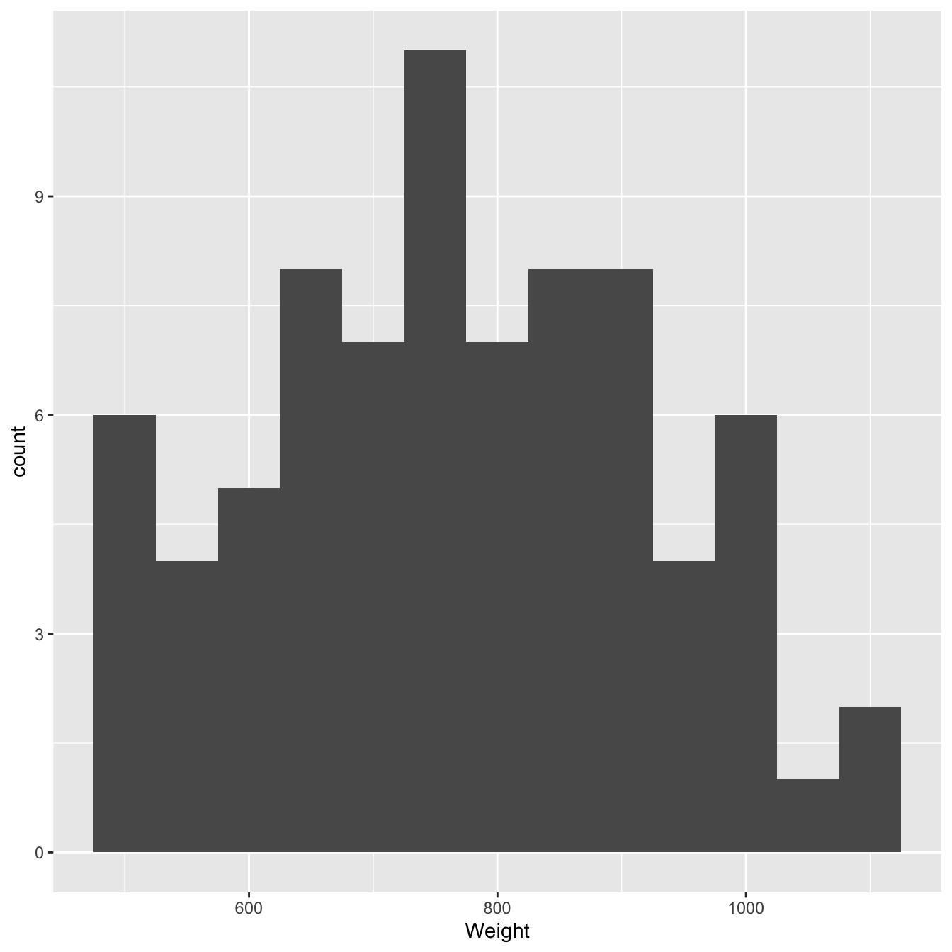

Figure 12.2: Size distributions of purple morph dry weight sample

These is nothing too ‘non-normal’ about this sample distribution—it’s roughly bell-shaped—so it seems reasonable to assume it came from normally distributed population.

12.3.2 Carrying out the test

It’s easy to carry out a one-sample t-test in R. The function we use is called t.test (no surprises there). Remember, Weight contains the dry weight biomass of purple plants. Here’s the R code to carry out a one-sample t-test:

t.test(purple_morphs$Weight, mu = 710)

We have suppressed the output because we want to initially focus on how to use the t.test function. We have to assign two arguments to control what the function does:

The first argument (purple_morphs$Weight) is simply a numeric vector containing the sample values. Sadly we can’t give t.test a data frame when doing a one-sample test. Instead, we have to pull out the column we’re interested in using the $ operator.
The second argument (called mu) sets the expected value we want to compare the sample mean to. So mu = 710 tells the function to compare the sample mean to a value of 710. This can be any value we like and the correct value depends on the question we’re asking.

That’s it for setting up the test. Here is the R code for the test again, this time with the output included:

t.test(purple_morphs$Weight, mu = 710)

## 
##  One Sample t-test
## 
## data:  purple_morphs$Weight
## t = 3.1811, df = 76, p-value = 0.002125
## alternative hypothesis: true mean is not equal to 710
## 95 percent confidence interval:
##  731.1490 801.9787
## sample estimates:
## mean of x 
##  766.5638

The first line tells us what kind of t-test we used. This says: One Sample t-test. OK, now we know that we used the one-sample t-test (there are other kinds). The next line reminds us about the data. This says: data: purple_morphs$Weight, which is R-speak for ’we compared the mean of the Weight variable to an expected value. Which value? This is given later.

The third line of text is the most important. This says: t = 3.1811, df = 76, p-value = 0.002125. The first part of this, t = 3.1811, is the test statistic, i.e. the value of the t-statistic. The second part, df = 76, summarise the ‘degrees of freedom.’ This is required to work out the p-value. It also tells us something about how much ‘power’ our statistical test has (see the box below). The third part, p-value = 0.002125, is the all-important p-value.

That p-value indicates that there is a statistically significant difference between the mean dry weight biomass and the expected value of 710 g (p is less than 0.05). Because the p-value is less than 0.01 but greater than 0.001, we report this as ‘p < 0.01.’ Read through the Presenting p-values section again if this logic is confusing.

The fourth line of text (alternative hypothesis: true mean is not equal to 710) tells us what the alternative to the null hypothesis is (H₁). More importantly, this serves to remind us which expected value was used to formulate the null hypothesis (mean = 710).

The next two lines show us the ‘95% confidence interval’ for the difference between the means. We don’t really need this information now, but we can think of this interval as a rough summary of the likely values of the ‘true’ mean⁴.

The last few lines summarise the sample mean. This might be useful if we had not already calculated.

A bit more about degrees of freedom

Degrees of freedom (abbreviated d.f. or df) are closely related to the idea of sample size. The greater the degrees of freedom associated with a test, the more likely it is to detect an effect if it’s present. To calculate the degrees of freedom, we start with the sample size and then we reduce this number by one for every quantity (e.g. a mean) we had to calculate to construct the test.

Calculating degrees of freedom for a one-sample t-test is easy. The degrees of freedom are just n-1, where n is the number of observations in the sample. We lose one degree of freedom because we have to calculate one sample mean to construct the test.

12.3.3 Summarising the result

Having obtained the result we now need to write our conclusion. We are testing a scientific hypothesis, so we must always return to the original question to write the conclusion. In this case the appropriate conclusion is:

The mean dry weight biomass of purple plants is significantly different from the expectation of 710 grams (t = 3.18, d.f. = 76, p < 0.01).

This is a concise and unambiguous statement in response to our initial question. The statement indicates not just the result of the statistical test, but also which value was used in the comparison. It is sometimes appropriate to give the values of the sample mean in the conclusion:

The mean dry weight biomass of purple plants (767 grams) is significantly different from the expectation of 710 grams (t = 3.18, d.f. = 76, p < 0.01).

Notice that we include details of the test in the conclusion. However, keep in mind that when writing scientific reports, the end result of any statistical test should be a conclusion like the one above. Simply writing t = 3.18 or p < 0.01 is not an adequate conclusion.

There are a number of common questions that arise when presenting t-test results:

What do I do if t is negative? Don’t worry. A t-statistic can come out negative or positive, it simply depends on which order the two samples are entered into the analysis. Since it is just the absolute value of t that determines the p-value, when presenting the results, just ignore the minus sign and always give t as a positive number.
How many significant figures for t? The t-statistic is conventionally given to 3 significant figures. This is because, in terms of the p-value generated, there is almost no difference between, say, t = 3.1811 and t = 3.18.
Upper or lower case The t statistic should always be written as lower case when writing it in a report (as in the conclusions above). Similarly, d.f. and p are always best as lower case. Some statistics we encounter later are written in upper case but, even with these, d.f. and p should be lower case.
How should I present p? There are various conventions in use for presenting p-values. We discussed these in the Hypotheses and p-values chapter. Learn them! It’s not possible to understand scientific papers or prepare reports properly without knowing these conventions.

p = 0.00? It’s impossible! p = 1e-16? What’s that?

Some statistics packages will sometimes give a probability of p = 0.00. This does not mean the probability was actually zero. A probability of zero would mean an outcome was impossible, even though it happened! When a computer package reports p = 0.00 it just means that the probability was ‘very small’ and ended up being rounded down to 0.

R typically uses a slightly different convention for presenting small probabilities. A very small probability is given as p-value < 2.2e-16. What does 2.2e-16 mean? This is R-speak for scientific notation, i.e. $2.2e^{-16}$ is equivalent to $2.2 \times 10^{-16}$.

Keep in mind that we should report a result like this as p < 0.001; do not write something like p = 2.2e-16.

It’s hard to say what constitutes a ‘large’ sample. If we’re lucky enough to be working with hundreds of observations it’s fine to ignore mild departures from normality. If we’re working with 10s of observations we probably need to pay a bit more attention to the normality assumption in a t-test.↩︎
In reality, a frequentist confidence interval is more complicated than that but this book probably isn’t the right place to get into that discussion. Take our word for it though—confidence intervals are odd things.↩︎