Chapter 11 Parametric statistics
11.1 Introduction
The majority of statistical tools used in this book share one important feature—they are underpinned by a mathematical model of some kind. Precisely because a mathematical model is lurking in the background, this particular flavour of statistics called parametric statistics. The word ‘parametric’ in this context refers to the fact that a mathematical model’s behaviour depends on one or more quantities known as ‘parameters.’
We are not going to study the mathematical details of these models. However, it is important to understand the assumptions underlying a statistical model. Assumptions are the aspects of a system that we accept as true, or at least nearly true. If our assumptions are not reasonable we can’t be sure that the results of our analysis (e.g. a statistical test) will be reliable. We always need to evaluate the assumptions of an analysis to determine whether or not we trust it.
Ultimately, we want to understand, in approximate terms, how a model and its assumptions lead to a particular statistical test. We have already explored aspects of this process in the last few chapters, such as sampling variation, null distributions, and p-values. By thinking about models and their assumptions we can begin to connect these abstract ideas to the practical side of ‘doing statistics.’ Our goal in this chapter is to introduce a few more concepts required to make these connections.
11.2 Mathematical models
A mathematical model is a description of a system using the language and concepts of mathematics. That ‘system’ could be more or less anything scientists study—the movement of planets in a solar systems, the carbon cycle of our planet, changes in abundance and distribution of a species, the development of an organ, or the spread of a plasmid conferring antibiotic resistance.
A statistical model—in the frequentist world, at least—is a type of mathematical model that describes how samples of data are generated from a hypothetical population. We’re only going to consider only a small subset of the huge array of statistical models people routinely use. Conceptually, the parametric models we use in this book describe data in terms of a systematic component and a random component:
\[\text{Observed Data} = \text{Systematic Component} + \text{Random Component}\] What are these two components?
The systematic component of a model describes the structure, or the relationships, in the data. When people refer to ‘the model,’ this is the bit they usually care about.
The random component captures the left over "noise" in the data. This is essentially the part of the data that the systematic component of the model fails to describe.
This is best understood by example. In what follows we’re going to label the individual values in the sample \(y_i\). The \(i\) in this label indexes the individual values; it takes values 1, 2, 3, 4, … and so on. We can think of the collection of the \(y_i\)’s as the variable we’re interested in.
The simplest kind of model we might consider is one that describes a single variable. A model for these data can be written: \(y_i = a + \epsilon_i\). In this model:
The systematic component is given by \(a\). This is usually thought of as the population mean.
The random component is given by \(\epsilon_i\), a term that describes how the individual values deviate from the mean.
A more complicated model is one that considers the relationship between the values of \(y_i\) and another variable. We’ll call this second variable \(x_i\). A model for these data could be written as: \(y_i = a + b \times x_i + \epsilon_i\). In this model:
The systematic component is the \(a + b \times x_i\) bit. This is just the equation of a straight line, with intercept \(a\) and slope \(b\).
The random component is given by the \(\epsilon_i\). Now this term describes how the individual values deviate from the line.
These two descriptions have not yet completely specified our example models. We need to make one more assumption to complete them. The values of the \(\epsilon_i\) differ from one observation to the next because they describe the noise in the system. For this reason, \(\epsilon_i\) is thought of as a statistical variable, which means we also need to specify its distribution.
What is missing from our description so far is, therefore, a statement about the distribution of the \(\epsilon_i\)—we need to formally set out what kinds of values it is allowed to take and how likely those different values are. In this book, this distributional assumption is almost always the same: we assume that the \(\epsilon_i\) are drawn from a normal distribution.
11.3 The normal distribution
Most people have encountered the normal distribution at one point or another, even if they didn’t realise it at the time. Here is a histogram of 100000 values drawn from a normal distribution:
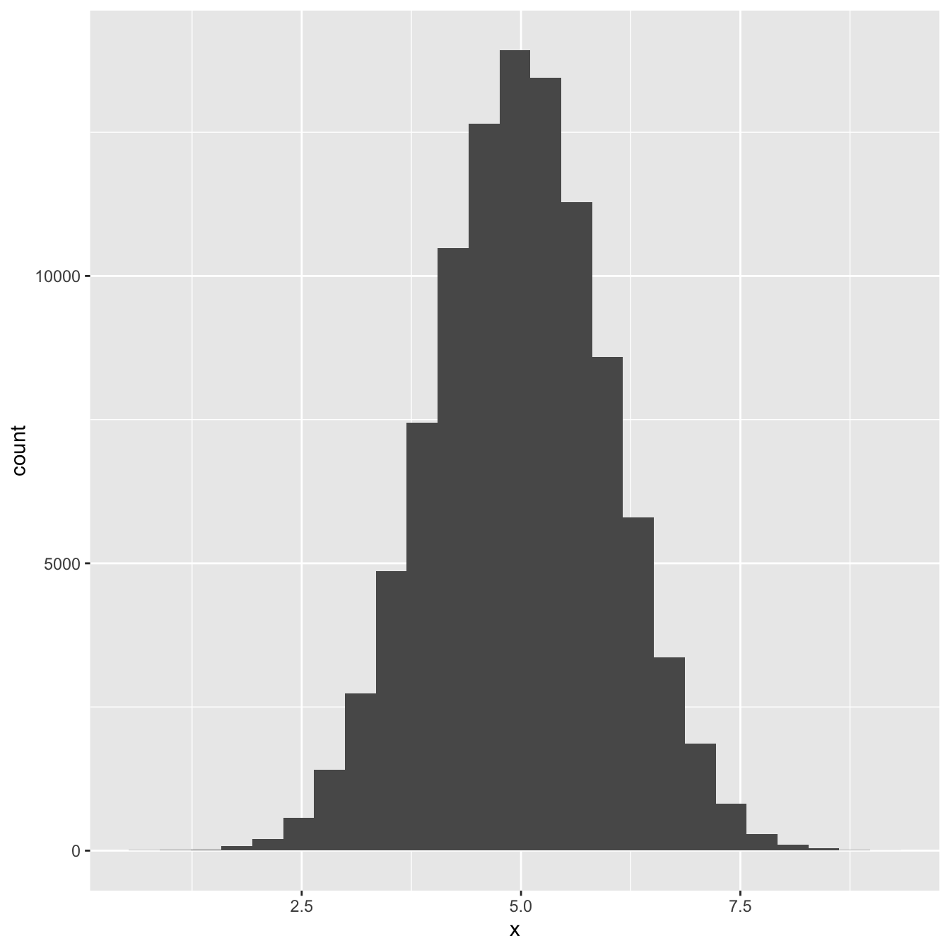
Figure 11.1: Distribution of a large sample of normally distributed variable
Does that look familiar? The normal distribution is sometimes called the ‘Gaussian distribution,’ or more colloquially, the ‘bell-shaped curve.’ We don’t have time in this book to study this distribution in any detail. Instead, we’ll simply list some key facts about the normal distribution that relate to the statistical models we’ll be using later on:
The normal distribution is appropriate for numeric variables measured on an interval or ratio scale. Strictly speaking, the variable should also be continuous, though a normal distribution can provide a decent approximation for some kinds of discrete numeric data.
The normal distribution is completely described by its mean (a measure of ‘central tendency’) and its standard deviation (a measure of ‘dispersion’). If we know these two quantities for a particular normal distribution, we know everything there is to know about that distribution.
If a variable is normally distributed, then about 95% of its values will fall inside an interval that is 4 standard deviations wide: the upper bound is equal to the \(\text{Mean} + 2 \times \text{S.D.}\); the lower bound is equal to \(\text{Mean} - 2 \times \text{S.D.}\).
When we add or subtract two normally distributed variables to create a new variable, the resulting variable will also be normally distributed. Similarly, if we multiply a normally distributed by a number to create a new variable, the resulting variable will still be normally distributed.
The mathematical properties of the normal distribution are very well understood. This has made it possible for mathematicians to work out how the sampling distribution of means and variances behave when the underlying variables are normally distributed. This knowledge underpins many of the statistical tests we use in this book.
11.3.1 Standard error of the mean
Let’s consider a simple example. We want to estimate the standard error associated with a sample mean. If we’re happy to assume that the sample was drawn from a normal distribution, then there’s no need to resort to computationally expensive techniques like bootstrapping to work this out.
There is a well-known formula for calculating the standard error once we assume normality. If \(s^2\) is the variance of the sample, and \(n\) is the sample size, the standard error is given by:
\[\text{Standard error of the mean} = \sqrt{\frac{s^2}{n}}\]
That’s it, if we know the variance and the size of a sample, it’s easy to estimate the standard error of its mean if we’re happy to assume the sample came from a normally distributed variable1.
In fact, as a result of rule #4 above, we can calculate the standard error of any quantity that involves adding or subtracting the means of samples drawn from normal distributions.
11.3.2 The t distribution
The normal distribution is usually the first distribution people learn about in a statics course. The reasons for this are:
it crops up a lot as a consequence of something called ‘the central limit theorem,’ and
many other important distributions are related to the normal distribution in some way.
We’re not going to worry about the central limit theorem here. However, we do need to consider one more distribution. One of the most important of those ‘other distributions’ is Student’s t-distribution2.
This distribution arises whenever…
we take a sample from a normally distributed variable,
estimate the population mean from the sample,
and then divide the mean by its standard error (i.e. calculate: mean / s.e.).
The sampling distribution of this new quantity has a particular form. It follows a Student’s t-distribution.
Student’s t-distribution arises all the time in relation to means. For example, what happens if we take samples from a pair of normal distributions, calculate the difference between their estimated means, and then divide this difference by its standard error? The sampling distribution of the scaled difference between means also follows a Student’s t-distribution.
Because it involves rescaling a mean by its standard error, the form of a t-distribution only depends on one thing: the sample size. This may not sound like an important result, but it really is, because it allows us to construct simple statistical tests to evaluate differences between means. We’ll be relying on this result in the next two chapters as we learn about so-called ‘t-tests.’
In fact, the equation for the standard error of a mean applies when we have a big sample, even if that sample did not come from a normally distributed variable. This result is a consequence of that ‘the central limit theorem’ mentioned in this chapter.↩︎
Why is it called Student’s t? The t-distribution was discovered by W.G. Gosset, a statistician employed by the Guinness Brewery. He published his statistical work under the pseudonym of ‘Student,’ because Guinness would have claimed ownership of his work if he had used his real name.↩︎