Chapter 14 Correlation
14.1 Introduction
The t-tests we encountered in the last two chapters were concerned with how to compare mean(s) of numeric variables. We learned how to: (1) compare one mean to any particular value via the one-sample t-test, (2) compare means among two groups or conditions via the two-sample t-test. One way to think about the two-sample t-tests is that they evaluate whether or not the variable changes among two groups or experimental conditions. Membership of the different groups/conditions can be encoded by a categorical variable. In R, we use a formula involving the numeric (num_var) and categorical (cat_var) variables to set up the test (e.g. num_var ~ cat_var). The formula reflects the fact that we can conceptualise the t-tests as considering a relationship between a numeric and categorical variable5.
In this chapter we’ll move on to discuss correlations, which are statistical measures that quantify an association between two numeric variables. An association is any relationship between the variables that makes them dependent in some way: knowing the value of one variable gives you information about the possible values of the second variable. The terms association and correlation are often used interchangeably, but strictly speaking correlation has a narrower definition. A correlation quantifies, via a correlation coefficient, the degree to which an association tends to a certain pattern.
There are a variety of methods for quantifying correlation, but these all share common properties:
- If there is no relationship between the variables then the correlation coefficient will be zero. The closer to 0 the value, the weaker the relationship. A perfect correlation will be either -1 or +1, depending on the direction. This is illustrated below…
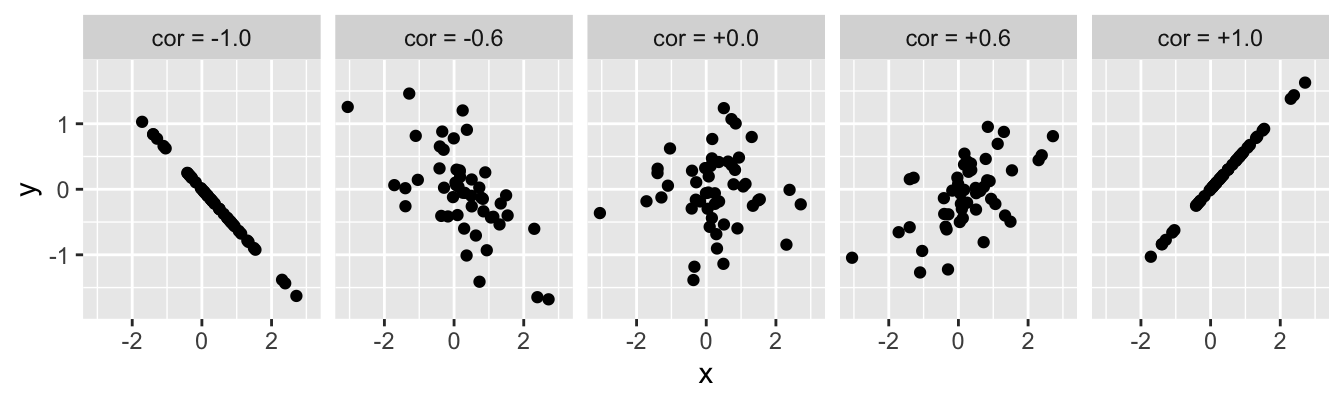
The value of a correlation coefficient indicates the direction and strength of the association, but says nothing about the steepness of the relationship. A correlation coefficient is just a number, so it can not tell us exactly how one variable depends on the other.
A correlation coefficient doesn’t tell us whether an apparent association is likely to be real or not. It is possible to construct a statistical test to evaluate whether a correlation is different from zero. Like any statistical test, this requires certain assumptions about the variables to be met.
There are several different measures of correlation between two variables. Here, we will consider probably the most commonly used method, Pearson’s product-moment correlation (\(r\)), often called Pearson’s correlation for convenience6:
14.2 Pearson’s product-moment correlation coefficient
Pearson’s correlation, being a parametric technique, makes some reasonably strong assumptions:
The data are on an interval or ratio scale.
The relationship between the variables is linear.
Both variables are normally distributed in the population.
The requirements are fairly simple and shouldn’t need any further explanation. It is worth making one comment though. Strictly speaking, only the linearity assumption needs to be met for Pearson’s correlation coefficient (\(r\)) to be a valid measure of association. As long as the relationship between two variables is linear, \(r\) produces a sensible measure. However, if the first two assumptions are not met, it is not possible to construct a valid significance test via the standard ‘parametric’ approach. In this course we will only consider the Pearson’s correlation coefficient in situations where it is appropriate to rely on this approach to calculate p-values. This means the first two assumptions need to be met.
We’ll work through an example to learn about Pearson’s correlation.
14.2.1 Pearson’s product-moment correlation coefficient in R
Bracken fern (Pteridium aquilinum) is a common plant in many upland areas. One concern is whether there is any association between bracken and heather (Calluna vulgaris) in these areas. To determine whether the two species are associated, an investigator sampled 22 plots at random and estimated the density of bracken and heather in each plot. The data are the mean Calluna standing crop (g m-2) and the number of bracken fronds per m2.
The data are in the file BRACKEN.CSV. Read these data into a data frame, calling it bracken:
## Rows: 22
## Columns: 2
## $ Calluna <int> 980, 760, 613, 489, 498, 416, 589, 510, 459, 680, 471, 145, 2…
## $ Bracken <dbl> 2.3, 1.4, 4.0, 3.6, 4.3, 4.0, 6.3, 6.5, 8.3, 8.2, 8.1, 9.1, 8…
There are only two variables in this data set: Calluna and Bracken. The first thing we should do is summarise the distribution of each variable:
ggplot(bracken, aes(x = Calluna)) + geom_dotplot(binwidth = 100)
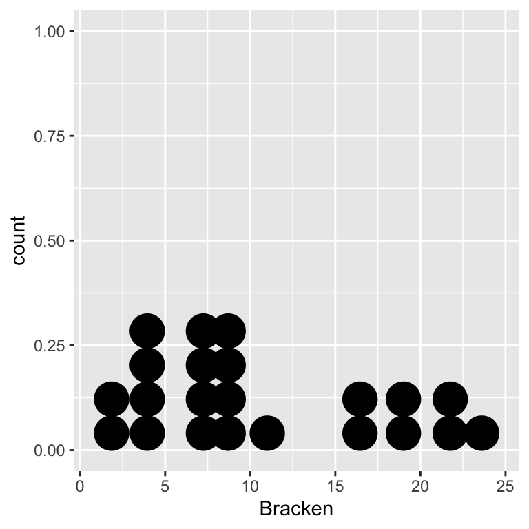
ggplot(bracken, aes(x = Bracken)) + geom_dotplot(binwidth = 2)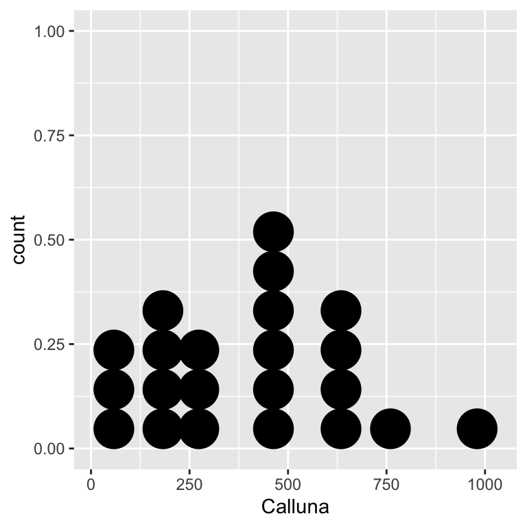
It looks like we’re dealing with numeric variables (ratio scale), each of which could be normally distributed. What we really want to assess is the association. A scatter plot is obviously the best way to visualise this:
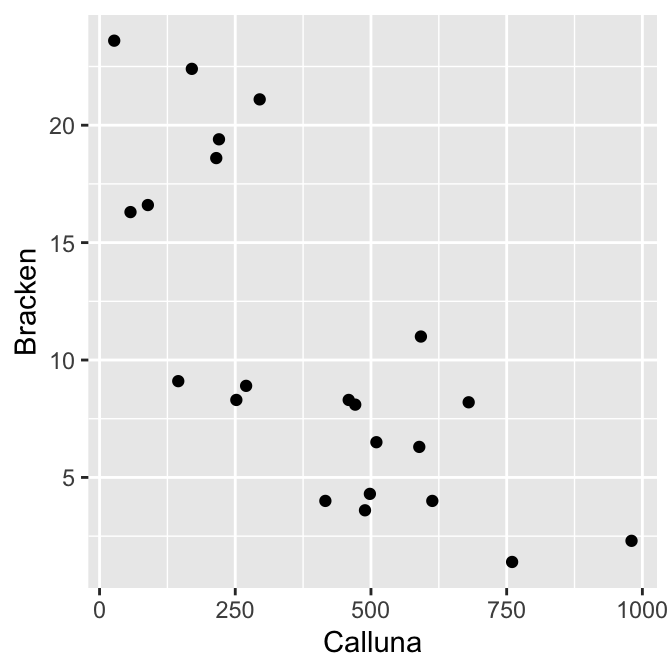
It seems clear that the two plants are negatively associated, but we should confirm this with a statistical test. We’ll base this on Pearson’s correlation.
Are the assumptions met? The scatter plot indicates that the relationship between the variables is linear, so Pearson’s correlation is a valid measure of association. Is it appropriate to carry out a significance test though? The data are of the right type—both variables are measured on a ratio scale—and the two dot plots above suggest the normality assumption is reasonable.
Let’s proceed with the analysis… Carrying out a correlation analysis in R is straightforward. We use the cor.test function to do this:
##
## 	Pearson's product-moment correlation
##
## data:  Calluna and Bracken
## t = -5.2706, df = 20, p-value = 3.701e-05
## alternative hypothesis: true correlation is not equal to 0
## 95 percent confidence interval:
##  -0.8960509 -0.5024069
## sample estimates:
##        cor
## -0.7625028
We use method = "pearson" to control which kind of correlation coefficient was calculated. There are three options, and although the default method is Pearson’s correlation, it is a good idea to be explicit. We use R’s formula system to determine which pair of variables are analysed. However, instead of placing a variable on the left hand side and a variable on the right hand side (e.g. Calluna ~ Bracken), both two variables appear to the right of the ~ separated by a + symbol. This convention makes good sense if you think about where we use correlation: a correlation analysis examines association, but it does not imply the existence of predictor and response variables. To emphasise the fact that neither variable has a special status, the cor.test function expects both variables to appear to the right of the ~, with nothing on the left.
The output from the cor.test is very similar to that produced by the t.test function. We won’t step through most of this output, as its meaning should be clear. The t = -5.2706, df = 20, p-value = 3.701e-05 line is the one we care about. Here are the key points:
The first part says that the test statistic associated with a Pearson’s correlation coefficient is a type of t-statistic. We’re not going to spend time worrying about where this came from, other than to note that it is interpreted in exactly the same way as any other t-statistic.
Next we see the degrees of freedom for the test. Can you see where this comes from? It is \(n-2\), where \(n\) is the sample size. Together, the degrees of freedom and the t-statistic determine the p-value…
The t-statistic and associated p-value are generated under the null hypothesis of zero correlation (\(r = 0\)). Since p < 0.05, we conclude that there is a statistically significant correlation between bracken and heather.
What is the actual correlation between bracken and heather densities? That’s given at the bottom of the test output: \(-0.76\). As expected from the scatter plot, there is quite a strong negative association between bracken and heather densities.
14.2.2 Reporting the result
When using Pearson’s method we report the value of the correlation coefficient, the sample size, and the p-value7. Here’s how to report the results of this analysis:
There is a negative correlation between bracken and heather among the study plots (r=-0.76, n=22, p < 0.001).
Notice that we did not say that bracken is having a negative effect on the heather, or vice versa.
It is perfectly possible to evaluate differences among means in more than two categories, but we don’t use t-tests to do this. Instead, we us a more sophisticated tool called Analysis of Variance (ANOVA). We’ll learn about ANOVA in later chapters.↩︎
People sometimes just refer to ‘the correlation coefficient’ without stating which measure they are using. When this happens, they probably used the most common method: Pearson’s product-moment correlation.↩︎
People occasionally report the value of the correlation coefficient, the t-statistic, the degrees of freedom, and the p-value. We won’t do this.↩︎