Chapter 9 Comparing populations
9.1 Making comparisons
Scientific inquiry requires that we evaluate our predictions about natural or experimentally-induced differences between populations. The simplest case involves just two populations, e.g.
‘Does enzyme activity differ among control and drug-treated cell lines?’
‘Do maize plants photosynthesise at different rates at 25°C and 20°C?’
‘Do purple and green plants differ in their biomass?’
In this setting we’re evaluating whether or not two populations are different in some way. To do this, we have to step through the same kind of process discussed in the last few chapters. This chapter demonstrates how to compare two populations by employing ideas like null hypotheses and p-values. The goal is not really to learn how to compare populations. Instead, we want to continue learning how these ideas are used to construct significance tests and evaluate predictions. On the way we’re going to introduce something called a ‘test statistic’.
9.1.1 A new example
We’ll continue with the now-familiar purple and green plants. However, instead of working with morph frequencies, this time we’ll consider plant size. We’ll introduce this new example by stepping through the process introduced in the learning from data chapter.
Question, hypothesis and prediction: We think there purple and green morph might be different in some way. Specifically, we want to address the question: Why have the purple morphs seemingly increased in frequency in the new study population? Based on the various observations already discussed, our working hypotheses is that purple plants are fitter than green plants. Since fitness is closely related to seed production, and seed production is typically positively correlated with plant size, we predict that purple morphs will be larger in the new population.
Statistical populations: What are the statistical populations we are interested in? This time we will conceive of each morph as its own population—i.e. there are now two statistical populations in play. This change of focus from our earlier analysis of this system is perfectly valid. Remember, statistical populations are not really fixed things. They are defined by the problem we’re working on.
Variables: Which variable should we study? An obvious way to address the prediction of size differences would be to measure the weight of individuals of each morph in our samples. In fact, ‘dry weight biomass’ is a very standard and reliable measure of how ‘big’ a plant is. Dry weight is a numeric variable, measured on a ratio scale (zero really does mean ‘nothing’).
Population porameters: Our prediction is that purple morphs will be larger than green morphs. What do we really mean by that? We probably don’t mean that every purple plant is bigger than every green plant. Instead, we want to know if purple plants are generally bigger than green ones. This can be thought of as a statement about ‘central tendency’—we want to evaluate whether purple plants are larger than green plants, on average. The population parameters of interest are therefore the mean dry weights of each morph.
Gather samples: The next step is to gather appropriate samples. Since this is a made-up example we’ll cut to the chase. We’ve already seen the samples we’re going to use. When we read in the ‘MORPH_DATA.CSV’ in the previous chapter we found it contained a numeric variable called Weight. This contains our dry weight biomass information. The categorical Colour variable analysed in the previous chapter tells us which kind of colour morph each observation corresponds to.
We’re now ready to tackle the remaining steps in the ‘learning from data’ process: estimating the population parameter(s), estimate uncertainty and answer the question. We’ll work through these remaining steps in detail next.
Once again, best way to understand what follows is to actually work through the example. And again, you are encouraged to do this…
9.1.2 Examine the data
You can carry on using the script you developed in the last chapter or set up a new project. Either way, for the code below to work you will need to have downloaded the ‘MORPH_DATA.CSV’ data file and read this into R, assigning it the name morph_data. Remember to check the data set again with str or glimpse.
The first step is to calculate point estimates of the mean dry weight of each morph. These are our ‘best guess’ of the population means. It will also be useful to know something about the sample size and variability of dry weight in each sample. We can summarise variability using the standard deviation (sd) of each sample. Here is how to do this with dplyr:
# using morph data...
morph_data %>%
  # ...group the data by colour morph category
  group_by(Colour) %>%
  # ... calculate the mean, sd and sample size of weight in each category
  summarise(mean = mean(Weight),
            sd = sd(Weight),
            samp_size = n())
## # A tibble: 2 x 4
## Colour mean sd samp_size
## <chr> <dbl> <dbl> <int>
## 1 Green 708. 150. 173
## 2 Purple 767. 156. 77This shows that the mean dry weight of the purple morph is indeed greater than that of green morph. Maybe our hypothesis is true. The standard deviation estimates indicate that the dry weight of purple morphs is also a bit more variable than the green morphs.
Remember, these numbers are point estimates derived from limited samples. If we sampled the populations again, sampling variation would lead to a different set of estimates. We’re not yet in a position to conclude that purple morphs are bigger than green morphs. To do this, we need to employ a statistical test to evaluate the significance of the mean differences.
We’ll evaluate that statistical significance in the next section. First, we need to visualise the the sample distributions of the weights of each colour morph. We could do this in a variety of ways. As we only have two samples we may as well use a fairly detailed summary. Histograms are a good choice when we have a reasonable amount of data:
ggplot(morph_data, aes(x = Weight)) +
  geom_histogram(binwidth = 50) +
  facet_wrap(~Colour, ncol = 1) # <- separate hist for each colour morph!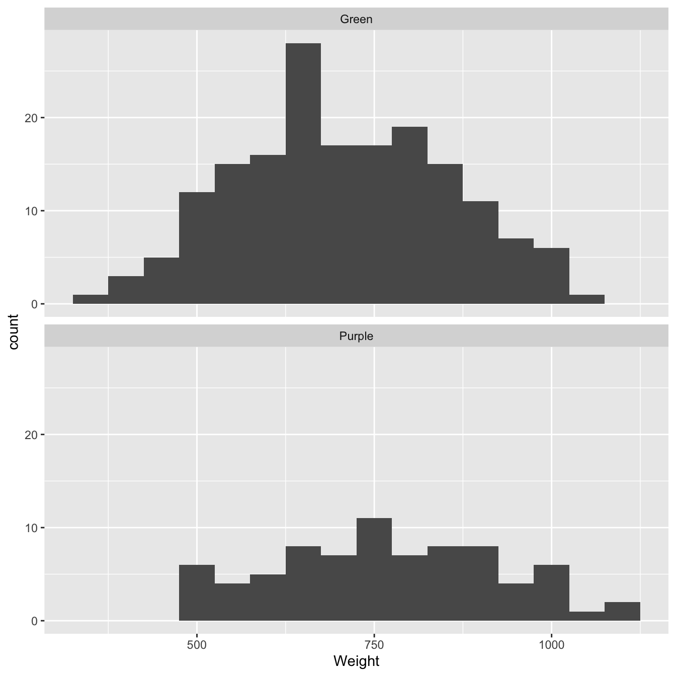
Figure 9.1: Size distributions of purple and green morph samples
What does this figure tell us? We’re interested in the degree of similarity of the two samples. It looks like purple morph individuals tend to have higher dry weights than green morphs. We already knew this but the plot confirms the difference has not resulted from a few extreme cases (‘outliers’).
So… the histograms confirm that there does seem to be a general difference in the size of the two morphs. However, there is also a lot of overlap between the two dry weight distributions. Maybe the difference between the sample means is just a result of sampling variation? It’s time to use a statistical test…
9.2 Constructing a test
We’re going to apply frequentist ideas to evaluate whether the two population means are likely to be different. We have to work through a four-step process to do this:
First, we assume there is really no difference between the population means. That is, we hypothesize that all the data are sampled from a pair of populations that have the same population mean. To put it another way, we pretend there is really only one population. We know about this trick. It’s a statement of the null hypothesis.
Next, we use information in the samples to work out what would happen if we were to repeatedly take samples in this hypothetical situation of ‘no difference between samples’. We summarise this by calculating the null distribution of some kind of test statistic
We then ask, “if there were no difference between the two groups, what is the probability that we would observe a difference that is the same as, or more extreme than, the one we observed in the true sample?” We know about this number too. It’s a p-value.
If the observed difference is sufficiently improbable, then we conclude that we have found a statistically significant result. A statistically significant result is one that is inconsistent with the hypothesis of no difference.
You will notice this logic is very similar to that used to construct a statistical test in the previous chapter. The only new elaboration here is the idea of the test statistic. When dealing with comparisons involving more than one parameter we have to work with a single numeric summary of the effect of interest (e.g. a difference between several means). The job of this quantity is to summarise the effect as a single number so that we can construct a test. That’s why the quantity is called the ‘test statistic’.
There are many different ways to go about realising this process above. We’re going to use something called a permutation test here. We’re not using this because we want you to learn how to apply it yourself. Instead, just as with the bootstrap, permutation tests offers a simple way to see how frequentist tests work without getting lost in mathematical detail.
9.2.1 Permutation tests
A hypothesis of ‘no difference’ between the mean dry weights of purple and green morphs implies the following: the labels ‘purple’ and ‘green’ are meaningless because the two morphs are effectively sampled from the same population. These labels don’t carry any real information so they may as well have been randomly assigned to each individual.
This suggests we can evaluate the statistical significance of the observed difference as follows:
- Make a copy of the original sample of purple and green dry weights, but do so by randomly assigning the labels ‘purple’ and ‘green’ to this new copy of the data. Do this in such a way that the original sample sizes are preserved. The process of assigning random labels is called permutation.
(We have to preserve the original sample sizes because we want to mimic the sampling process that we actually used, i.e. we want to hold everything constant apart from the labelling of individuals.)
Repeat the permutation scheme many times until we have a large number of artificial samples; 1000-10000 randomly permuted samples may be sufficient.
For each permuted sample, calculate whatever test statistic captures the relevant information. In our example, this is the difference between the mean dry weight of purple and green morphs in each permuted sample.
(It doesn’t matter which way round we calculate the difference.)
- Compare the observed test statistic from the real sample to the distribution of sample statistics from the randomly permuted samples.
This scheme is called a permutation test because it involves random permutation of the group labels. Why is this useful? Each unique random permutation yields an observation from the null distribution of the difference among sample means, under the assumption that this difference is really zero in the population. We can use this to assess whether or not the observed difference is consistent with the hypothesis of no difference by looking at where it lies relative to this null distribution.
9.2.2 Carrying out a permutation test
It’s ease to implement a permutation test in R. We won’t show the code this time because it uses quite a few tricks that won’t be needed again. It is worth having a quick look at the permuted samples though. The first 40 values from two permuted samples are:
Sample 1-
##     Green    Purple    Purple     Green     Green    Purple     Green    Purple
##  714.3592  693.4924  556.2063  653.6619  672.5207  661.0097  445.1001  481.5068
##     Green     Green     Green     Green    Purple    Purple     Green     Green
##  647.6679  858.4820  567.4104  597.1629  718.7132  539.8551  753.0170  807.7700
##    Purple    Purple     Green     Green     Green     Green     Green     Green
## 1085.7036  926.4972  617.1209  632.5897  859.7013  815.4634  666.7693  573.5907
##     Green     Green    Purple     Green    Purple    Purple     Green     Green
##  694.2877  836.6883  665.8489  617.7895  590.5936  775.8980  686.6790  813.4272
##     Green     Green     Green    Purple     Green     Green     Green    Purple
##  506.3904  566.9971  629.5894  878.2477  823.1128  542.7877  507.7345  786.2809
Sample 2-
##    Purple     Green     Green     Green     Green     Green    Purple    Purple
##  714.3592  693.4924  556.2063  653.6619  672.5207  661.0097  445.1001  481.5068
##    Purple     Green     Green    Purple    Purple     Green    Purple     Green
##  647.6679  858.4820  567.4104  597.1629  718.7132  539.8551  753.0170  807.7700
##    Purple     Green     Green     Green    Purple    Purple     Green    Purple
## 1085.7036  926.4972  617.1209  632.5897  859.7013  815.4634  666.7693  573.5907
##    Purple     Green     Green    Purple     Green     Green     Green     Green
##  694.2877  836.6883  665.8489  617.7895  590.5936  775.8980  686.6790  813.4272
##    Purple     Green     Green     Green    Purple     Green     Green    Purple
##  506.3904  566.9971  629.5894  878.2477  823.1128  542.7877  507.7345  786.2809
The data from each permutation are stored as numeric vectors, where each element of the vector is named according to the morph type it corresponds to—these are ‘the labels’ referred to above. The set of numbers does not vary among permuted samples. The only difference between them is the labelling which has been randomly assigned in each permuted sample.
The difference between the mean dry weights in the first permutation is 4.0700017, while in the second sample, the difference is -19.9656492. What matters for our test is the distribution of these differences over the complete set of permutations. This is the approximation to the sampling distribution of the difference between means under the null hypothesis—i.e. it’s our null distribution.
We can visualise this null distribution by making a histogram that summarises the 2500 mean differences from the permuted samples:
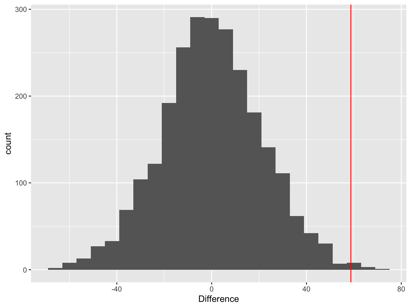
Figure 9.2: Difference between means of permuted samples
Notice that the distribution is centred at zero. This makes perfect sense—if we take a set of numbers and randomly allocate them to groups, on average, we expect the difference between the means of the groups to be zero.
The red line shows the estimated value of the difference between the mean purple and green morph dry weights in the real sample. This is the test statistic. The key thing to notice here is the location of the test statistic within the null distribution.
In this example, the estimated difference lies at the end of the right ‘tail’ of the null distribution. What does that tell us? It suggests the observed difference (the red line) is unlikely to arise through pure sampling variation when the population means of the two groups really were identical.
So… it looks like the data are inconsistent with the null hypothesis of no difference. What we need is a number to quantify this inconsistency—the p-value.
Calculating the p-value
We can use the null distribution to quantify the probability of ending up with the observed difference under the null hypothesis. Only 10 out of the 2500 permutations ended up being equal to, or ‘more extreme’ (more positive) than, the observed difference. The probability of finding a difference in the means equal to, or more positive than, the observed difference is therefore, p = 10/2500 = 0.004. This is the p-value associated with our significance test.
Let’s run through the interpretation of that p-value. Here’s the general chain of logic again… The p-value is the probability of obtaining a test statistic equal to, or ‘more extreme’ than, the estimated value, assuming the null hypothesis is true. The null hypothesis is one of no effect, so a small p-value can be interpreted as evidence for the effect (e.g. a difference between means) being present. That’s a weird way to seek evidence for the presence of an effect but that’s how frequentist statistics works.
How low does the p-value actually have to be before we decide we have ‘enough evidence’? Less than 0.01? Less than 0.001? Any threshold is somewhat arbitrary to be honest, but in biology, a significance threshold of p < 0.05 is conventionally used. If we find p < 0.05, then we conclude that we found a ‘statistically significant’ effect at the 5% level.
Here’s how this logic applies to our example… The permutation test assumed there was no difference between the purple and green morphs, so the low p-value indicates that the estimated difference between the mean dry weight of purple and green morphs was unlikely to have occurred by chance if there is really no difference at the population level. We interpret the low p-value as evidence for the existence of a difference in mean dry weight among the populations of purple and green morphs. Since p = 0.004, we say we found a statistically significant difference at the 5% level.
Directional tests
The test we just did is a ‘one-tailed’ test. It’s called a ‘one-tailed’ because we only looked at one end of the null distribution. This kind of test is appropriate for evaluating directional predictions (e.g. purple > green). If, instead of testing whether purple plants were larger than green plants, we just want to know if they were different in some way (i.e. in either direction), we should use a ‘two-tailed’ test. These work by looking at both ends of the null distribution. We won’t do this here though—the one- vs two-tailed distinction is discussed in the one-tailed vs. two-tailed tests supplementary chapter.
Here’s how we might summarise our analysis in in a written report:
The mean dry weight biomass of purple plants (77) was significantly greater than that of green plants (173) (one-tailed permutation test, p<0.05).
We report the sample sizes used, the type of test employed, and the significance threshold we passed (not the raw p-value).
9.3 What have we learned?
Our goal was not really to learn how permutation tests work. Just as with bootstrapping in the previous chapter—we just used it to demonstrate the logic of how frequentist statistics work. In this instance, we wanted to see how to evaluate a difference between two groups. The basic ideas are no different from those introduced in the previous chapter…
define what constitutes an ‘effect’ (e.g. a difference between means), then assume that there is ‘no effect’—i.e. define the null hypothesis,
select an appropriate test statistic that can distinguish between the presence of an ‘effect’ and ‘no effect’,
(In practice, each kind of statistical test uses a standard test statistic. We don’t have to pick these ourselves.)
construct the corresponding null distribution of the test statistic by working out what would happen if we were to take frequent samples in the ‘no effect’ situation,
and finally, use the null distribution and the observed test statistic to calculate a __p-value__that quantifies how frequently the observed difference, or a more extreme difference, would be observed under the hypothesis of no effect.
We only actually introduced one new idea in this chapter. When evaluating differences among populations we need to work with a single number that can distinguish between ‘effect’ and ‘no effect’. This is called the test statistic. Sometimes this can be expressed in terms of familiar quantities like means (we just used a difference between means above). However, this isn’t always the case. For example, we can use something called an F-ratio to evaluate the statistical significance of differences among more than two means. We’ll get to these kinds of tests later. For now, our task is to explore simple ‘parametric tests’. These kinds of tests allow us to ask questions without resorting to things bootstrapping or permutation tests.